You can use VLOOKUP across multiple sheets in Google Sheets by first combining the ranges from different sheet tabs into a single virtual range and then applying VLOOKUP to that combined range.

However, when working with open-ended ranges, you should combine them carefully. Otherwise, the combined range may include thousands of unnecessary empty rows, which can negatively affect spreadsheet performance.

In this tutorial, you’ll learn the best way to use VLOOKUP across multiple sheets in Google Sheets with both closed and open-ended ranges.

Examples

If you’d like to follow along with the examples in this tutorial, make a copy of the sample sheet below.

Copy the Sample Sheet

VLOOKUP Across Multiple Sheets Using Closed Ranges

Suppose you have price lists for soups, non-vegetarian, and vegetarian items stored in three sheet tabs:

• 'New1'!B3:C6
• 'New2'!B3:C6
• 'New3'!B3:C6

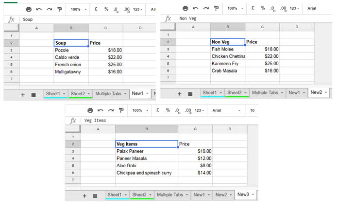
In another sheet, the search key (for example, “Crab Masala”) is in cell B2.

Use the following formula in cell C2:

=VLOOKUP(B2, VSTACK('New1'!$B$3:$C$6, 'New2'!$B$3:$C$6, 'New3'!$B$3:$C$6), 2, FALSE)

The VSTACK function combines the three ranges vertically into a single array. VLOOKUP then searches the first column of the combined array and returns the corresponding value from the second column.

Using Multiple Search Keys

If your search keys are in the range B2:B4, either drag the above formula down or wrap it with ARRAYFORMULA:

=ARRAYFORMULA(VLOOKUP(B2:B4, VSTACK('New1'!B3:C6, 'New2'!B3:C6, 'New3'!B3:C6), 2, FALSE))

This is the simplest way to use VLOOKUP across multiple sheets in Google Sheets when your source ranges have fixed boundaries.

VLOOKUP Across Multiple Sheets Using Open-Ended Ranges

When your source ranges are open-ended, such as B3:C, the combined array contains many blank rows. Filtering out those blank rows improves performance.

Use the following formula:

=LET(
  combine, VSTACK('New1'!$B$3:$C, 'New2'!$B$3:$C, 'New3'!$B$3:$C),
  ftr_combine,
    FILTER(combine, CHOOSECOLS(combine, 1)<>""),
  VLOOKUP(B2, ftr_combine, 2, FALSE)
)

Formula Explanation

combine

Uses VSTACK to combine the open-ended ranges into a single array.

ftr_combine

Uses FILTER to remove rows where the first column is blank. This significantly reduces the size of the lookup array and helps improve performance.

VLOOKUP

Searches for the value in B2 within the filtered array and returns the value from the second column.

Using Multiple Search Keys

To return results for multiple search keys, replace:

VLOOKUP(B2, ftr_combine, 2, FALSE)

with:

=ARRAYFORMULA(VLOOKUP(B2:B4, ftr_combine, 2, FALSE))

This is the recommended dynamic approach for using VLOOKUP across multiple sheets in Google Sheets with open-ended ranges.

Conclusion

In this tutorial, we covered two methods to use VLOOKUP across multiple sheets in Google Sheets.

• Use closed ranges when your data range is fixed.
• Use open-ended ranges together with FILTER when your data grows over time. Filtering out blank rows keeps the lookup array smaller and improves performance.

If you’re combining data from many sheet tabs (for example, more than 10), the formula can become quite long. In that case, a better approach is to store the sheet names in a column and combine the data dynamically based on that list.

You can learn that technique in my tutorial: Combine Data Dynamically in Multiple Tabs Vertically in Google Sheets.