This tutorial explains how to use the TOROW function in Google Sheets. Also, we can discuss one real-life use of this function.

The purpose of this newly introduced (2023) function in Sheets is to transform a range of cells into a single row.

It avoids using FLATTEN, TRANSPOSE, and FILTER combinations, a workaround solution to transform a table or array into a single row.

The combination function won’t be the cup of tea for many new Sheets users.

They may prefer standalone functions for data manipulation.

In that context, this new function will be a relief for many Sheets enthusiasts.

TOROW Function Syntax and Arguments

Syntax: TOROW(array_or_range, [ignore], [scan_by_column])

Arguments:

array_or_range — The array or cell range to return as a row.

ignore — Whether to ignore blanks (1), errors (2), or both (3). By default (0), no values are ignored. Specify 0, 1, 2, or 3 accordingly.

scan_by_column — TRUE (by column) or FALSE (by row [default]).

Here are a few examples of using the TOROW function in Google Sheets.

TOROW Function Examples in Google Sheets

Please see the values in the range B2:D6, which I’ve generated using the following SEQUENCE formula in B2: =sequence(5,3)

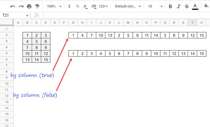
In G2, I’ve used a TOROW formula to scan these values by column.

=torow(B2:D6,0,true)

The G5 formula scans the values by row.

=torow(B2:D6,0,false)

Understand the difference, and you won’t falter in using the TOROW function in Google Sheets.

In both formulas, the ignore parameter is set to 0, which means returning the values as it is.

Alternative Solutions

You can ignore the below formulas. I just put it to show you how complex things were earlier.

G2:

=transpose(flatten(transpose(B2:D6)))

G5:

transpose(flatten(B2:D6))

One of the issues with these alternatives to the TOROW function is you may additionally require to use FILTER and IFERROR to ignore blanks, errors, or both.

TOROW Real-life Use: Inserting Blank Columns between Data

Sometimes we can better manipulate values in a range of cells in Sheets when it is in a single row or column.

We can use the TOROW function in Google Sheets for transforming the range of cells into a row.

After manipulating the values, with the help of WRAPROWS, we can transform the single rows of values back into the range of cells.

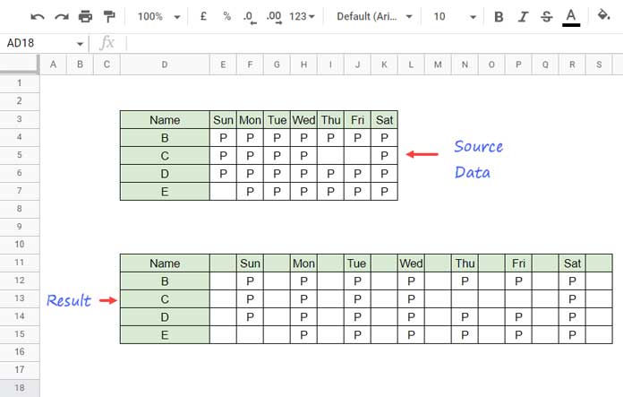
In the following examples, you can learn how to insert blank columns between data using a combination of TOROW and WRAPROWS functions in Google Sheets.

Similar: How to Insert Blank Columns in Google Sheets Query.

The following Google Sheets formula in cell D11 inserts blank columns between the source data in D3:K7.

=let(
     data,
     D3:K7,
     iferror(
          wraprows(
               torow(
                   {torow(data,0,false);
                    index(torow(data/0,0,false))
                   },
                   0,true
               ),
               columns(data)*2
          )
     )
)

How does the above formula be able to insert blank columns between data?

There are four key steps.

1. First, we should flatten the data into a row by scanning the values by row. So the scan_by_column is set to FALSE.

torow({torow(data,0,false)

2. The next step is to generate error cells matching the number of cells in the data range.

index(torow(data/0,0,false))

Then create an array in the following syntax: {step#1;step#2}

3. Use another TOROW to flatten this ‘new’ array into a row, but this time scan by column. So the scan_by_column is set to TRUE.

TOROW({step#1;step#2},0,true)

It will place one error value after every value.

4. Finally, the WRAPROWS creates an array.

Syntax: WRAPROWS(range, wrap_count, [pad_with])

Please note that the wrap_count is the number of columns in the data * 2.

This way, we can insert blank columns between data using WRAPROWS and TOROW functions in Google Sheets.