In this tutorial, we will check whether we can use SUMIF across multiple Sheets, or if not, what is the alternative in Google Sheets.

The SUMIF function operates well with a single range in a Sheet.

If you want to use it with multiple ranges, within a Sheet or from more than one Sheet within the workbook, you should first append those ranges across Sheets vertically in another Sheet.

You can use the VSTACK function for that. Here is the syntax of it.

Syntax: VSTACK(range1, [range2, …])

So there will be a new physical range to apply the SUMIF conditional sum. 

The function will return the ‘infamous’ “Argument must be a range” error in the absence of a physical range. Below is an example of this error state.

=sumif(
     vstack('April 23'!B2:B10,'May 23'!B2:B11),
     "Stationery",
     vstack('April 23'!C2:C10,'May 23'!C2:C11)
)

The above is an attempt to SUMIF across two Sheets. But returns #N/A because of the absence of a physical range.

So that left us with two options when we want to SUMIF across multiple Sheets in Google Sheets.

• Append the ranges in a new Sheet in the same workbook and use SUMIF in that NEW physical range.
• Use the formula in use for append ranges directly within a QUERY.

We will see examples of both these options below.

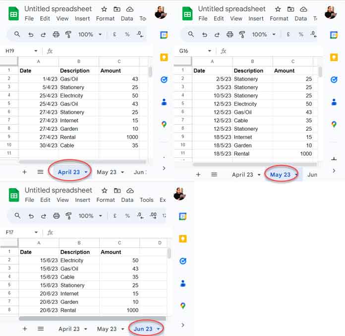
Sample Data: Daily Expense Sheets

Assume my daily expense data is spread across multiple Sheets within a workbook, and “Internet” is one of the categories (account head) of expense.

The daily data is in three Sheets: “April 23,” “May 23,” and “Jun 23.”

We will see how to use SUMIF across these Sheet tabs to total the expense incurred on the item “Internet.”

Append Ranges Across Sheets Vertically for SUMIF

We want to apply SUMIF across the ranges A1:C in Sheets “April 23,” “May 23,” and “Jun 23” within a workbook in Google Sheets.

The field labels are Date, Description, and Amount in A1:C1 (please refer to the screenshot above).

With the help of VSTACK, we can vertically append the ranges A2:C from these Sheets as below in a fourth Sheet named “Dashboard.”

We have used A2:C instead of A1:C to avoid titles in the combined range.

Formula (Dashboard!B1):

=LET(
     appended,
     VSTACK('April 23'!A2:C,'May 23'!A2:C,'Jun 23'!A2:C),
     FILTER(
          appended,
          TRIM(TRANSPOSE(QUERY(TRANSPOSE(appended),,9^9)))<>""
     )
)

Note:

The bold part in the above formula is only sufficient. But there might be hundreds of blank rows between each range appended.

The other part of the formula removes those blanks. You can read more about it here: Filter Out If the Entire Row Is Blank in Google Sheets.

We are ready to use SUMIF across multiple Sheets in Google Sheets. We will come to that under the next subtitle.

Before that, one more thing. Some of you may have the below question. Let me clarify that first.

I want to specify Sheet names in A1:A in the “Dashboard” Sheet and refer to that instead of hardcoding them within the VSTACK formula as above. How do we do that?

No problem. Use this code in Dashboard!B1 instead of the above VSTACK.

=LET(combined,LET(data,"A2:C",tabs,A1:A,REDUCE(HSTACK(IFERROR(INDEX(SEQUENCE(1,3)/0))),FILTER(tabs,tabs<>""),LAMBDA(accu,val,VSTACK(accu,INDIRECT(val&"!"&data))))),FILTER(combined,TRIM(TRANSPOSE(QUERY(TRANSPOSE(combined),,9^9)))<>""))

Where “A2:C” is the range to append and A1:A is the range containing the Sheet names.

Important:

When you enter the above Sheet names in A1:A, the application will read them as dates instead of texts because they contain month and year.

So first select the range A1:A and apply the menu command Format > Number > Plain text. Then start entering the Sheet names.

If the above formula drives you bananas, import and use my COPY_TO_MASTER_SHEET named function.

SUMIF Across Multiple Sheets in Google Sheets

Syntax: SUMIF(range, criterion, [sum_range])

We will now see how to use SUMIF across these Sheet tabs to total the expense incurred on the item “Internet.” It is as simple as below.

=sumif(Dashboard!C1:C,"Internet",Dashboard!D1:D)

If you prefer to enter the criterion Internet in cell E1 and refer to that in SUMIF, use the following formula.

=sumif(Dashboard!C1:C,Dashboard!E1,Dashboard!D1:D)

How to use more than one condition, e.g., “Cable” and “Internet,” when SUMIF across multiple sheets in Google Sheets?

SUMIF across multiple sheets formula when the conditions Internet in E1 and Cable in E2:

=ArrayFormula(sumif(Dashboard!C1:C,Dashboard!E1:E2,Dashboard!D1:D))

Here is the hardcoded way.

=ArrayFormula(sumif(Dashboard!C1:C,vstack("Internet","Cable"),Dashboard!D1:D))

Skipping the “Dashboard” Helper Sheet

Not everyone like an extra Sheet for SUMIF across multiple Sheets. For example, the “Dashboard” Sheet in our above formula.

If you are one such user, try this QUERY function alternative to SUMIF across multiple Sheets.

In this, replace append_formula with the Dashboard!B1 formula.

=QUERY(append_formula,"Select Col2,sum(Col3) where lower(Col2)='internet' group by Col2 label sum(Col3)''",0)

In this, the criterion is “Internet.” You must specify it in lowercase as the formula is case-sensitive.

Note:- Replace lower(Col2)='internet' with lower(Col2)='"&lower(Dashboard!E1)&"' for specifying a cell, here E1, that contains the criterion.

What about “Cable” and “Internet” as the criteria similar to the SUMIF across multiple Sheets formula?

=QUERY(append_formula,"Select Col2,sum(Col3) where lower(Col2) matches 'cable|internet' group by Col2 label sum(Col3)''",0)

Separate each criterion with a pipe separator (also please note the use of the MATCHES operator).

Note:- Replace 'cable|internet' with '"&textjoin("|",true,index(lower(Dashboard!E1:E2)))&"' for specifying a cell range, here E1:E2, that contains the criteria.

SUMIFS Across Multiple Sheets in Google Sheets

Syntax: SUMIFS(sum_range, criteria_range1, criterion1, [criteria_range2, …], [criterion2, …])

Like its sibling, the SUMIFS is also not for use across the Sheets.

We must first append the ranges in each Sheet as earlier. So we have the “Dashboard” Sheet with the appended data.

How do we code SUMIFS to return the total of “Cable” expenses for April and May?

The following SUMIFS will return the total expenses incurred in April and May.

=ArrayFormula(SUMIFS(Dashboard!D1:D,REGEXMATCH(MONTH(Dashboard!B1:B)&"","^4$|^5$"),TRUE))

With this, we can add the category “Cable” as follows.

=ArrayFormula(SUMIFS(Dashboard!D1:D,REGEXMATCH(MONTH(Dashboard!B1:B)&"","^4$|^5$"),TRUE,Dashboard!C1:C,"Cable"))

What about adding the categories “Cable” and “Internet”?

=ArrayFormula(SUMIFS(Dashboard!D1:D,REGEXMATCH(MONTH(Dashboard!B1:B)&"","^4$|^5$"),TRUE,REGEXMATCH(Dashboard!C1:C,"(?i)^Cable$|^Internet$"),TRUE))

As you can see, the REGEXMATCH plays a key role when more than one criterion is in one column.

Related: REGEXMATCH in SUMIFS and Multiple Criteria Columns in Google Sheets.