Like SQL, you can interact with a database-style array using the DMIN function in Google Sheets. All database functions in Google Sheets are designed for this purpose.

The DMIN function in Sheets returns the minimum value from a database-style array, similar to how a SQL query operates.

You may be unfamiliar with the term “database-style array” mentioned above. It refers to source data, or records, arranged in rows. However, like a database table, the first row of the range must contain labels representing the values in each column. In short, it’s a range with no merged cells and a header row, or it could be the new Google Sheets Table (Insert > Table).

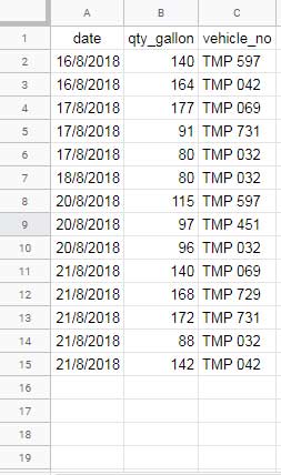
The above sample data shows the date-wise diesel consumption or refilling for a few vehicles. Notice that the first row contains column labels.

In data like this, you can use database functions, including DMIN, effortlessly.

If labels aren’t present, you may need to use MINIFS instead.

Syntax of the DMIN Database Function in Google Sheets:

DMIN(database, field, criteria)

Arguments:

• database – The range containing the data, which adheres to the database table-like array structure mentioned above.
• field – The column in the database to find the minimum value. You can use either the column label or the column number. The first column in the database is numbered 1.
• criteria – The condition used to filter the database.

Let me explain how to use the DMIN function in Google Sheets along with some tips for working with criteria.

Examples

Let’s consider the same sample data. The first column contains the fuel filling dates labeled ‘date’, the second column contains the filled quantities in gallons (qty_gallon), and the third column contains the vehicle numbers (vehicle_no). Below are tips on how to use criteria with this function.

DMIN Function and String Criteria in Sheets

The formula below returns the minimum fuel quantity filled by the vehicle “TMP 597”:

=DMIN(A1:C15, 2, {"vehicle_no"; "TMP 597"})

Alternatively, if you want to use a cell reference for the criterion, where E1 contains “vehicle_no” and E2 contains “TMP 597”, the formula will be:

=DMIN(A1:C15, 2, E1:E2)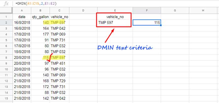

There are three common types of criteria: text, number, and date. Sometimes, you may also need to use comparison operators.

Above, I’ve demonstrated how to use text criteria in DMIN. Now, let’s explore a DMIN formula using a date as the criterion.

DMIN Function and Date Criteria in Sheets

This formula filters the rows that contain the date 17/08/2018 in the first column, and then finds the minimum value in the second field:

=DMIN(A1:C15, 2, {"date"; DATE(2018, 8, 17)})

The date is specified using the DATE function, with the syntax DATE(year, month, day).

Here’s the equivalent formula when E1 contains ‘date’ and E2 contains 17/08/2018:

=DMIN(A1:C15, 2, E1:E2)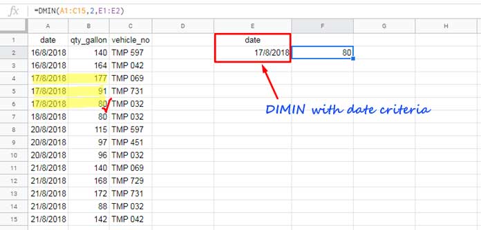

Similarly, you can use a TIME criterion. When hardcoding, use the time in the format TIME(hour, minute, second).

DMIN Function and Number Criteria in Sheets

For this example, we’ll use a new sample dataset with ‘Player Name’, ‘Matches’, and ‘Goals’ as field labels. The data range is A1:C6.

In the following DMIN formula, E1 and E2 contain “Matches” and 5, respectively:

=DMIN(A1:C6, 3, E1:E2)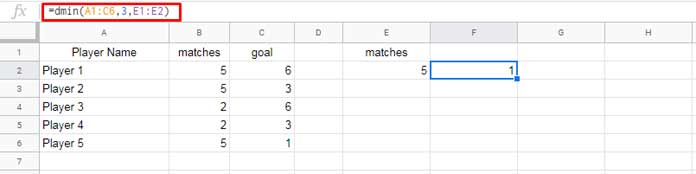

The formula returns the least number of goals scored by any player in 5 matches. Alternatively, the formula can be hardcoded as:

=DMIN(A1:C6, 3, {"Matches"; 5})

DMIN Formula with Comparison Operators

Here’s an example of using a comparison operator with the DMIN function for a numeric criterion in Google Sheets:

=DMIN(A1:C6, 3, {"matches"; ">4"})

When referring to a cell, you can directly type the criteria with the comparison operator:

For instance, if E1 contains “matches” and E2 contains “>4”, use:

=DMIN(A1:C6, 3, E1:E2)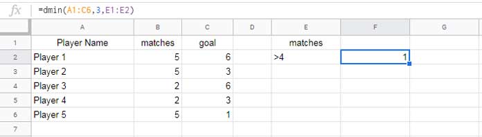

This approach also applies to date fields.

Additional Tips: No Criteria and Multiple Criteria Usage

In the examples above, we used a single criterion. But what if you don’t want to specify any criterion?

To exclude criteria, you can simply specify the field label and leave an empty cell below it. Refer to this range in the formula.

When hardcoding, you can specify criteria using two empty cells, such as {IF(,,); IF(,,)}.

For multiple criteria from two different fields, enter the field labels in E1:F1 and the relevant criteria below them.

If you have multiple criteria for the same field, enter the field label in E1 and list the criteria below it, one after another.

For hardcoding multiple criteria, please refer to: The Ultimate Guide to Using Criteria in Database Functions in Google Sheets.

Resources

• Row-Wise MIN Using DMIN in Google Sheets
• Get Min Date Ignoring Blanks in Each Row in Google Sheets
• Find the Running Minimum Value in Google Sheets
• Exact Match in Database Functions in Google Sheets – How-To