Click on a link label to jump to that cell! This post shed some light on how to hyperlink to max and min values in a single column as well as in a single row in Google Sheets. This is possible by finding the cell address of max/large or min/small values.
Max and Large are the two functions to find max values. The opposite functions are Min and Small. I am ignoring the Database functions for the same that starts with the letter “D”, for example, Dmin.
Assume I have used the following Max formula in cell C1 to return the max value from column A.
=max(A1:A)The output, as per the sample list (A1:A) below, is 100. How to jump to that max result cell?
Hyperlink to Jump to Max Value Column in Google Sheets:
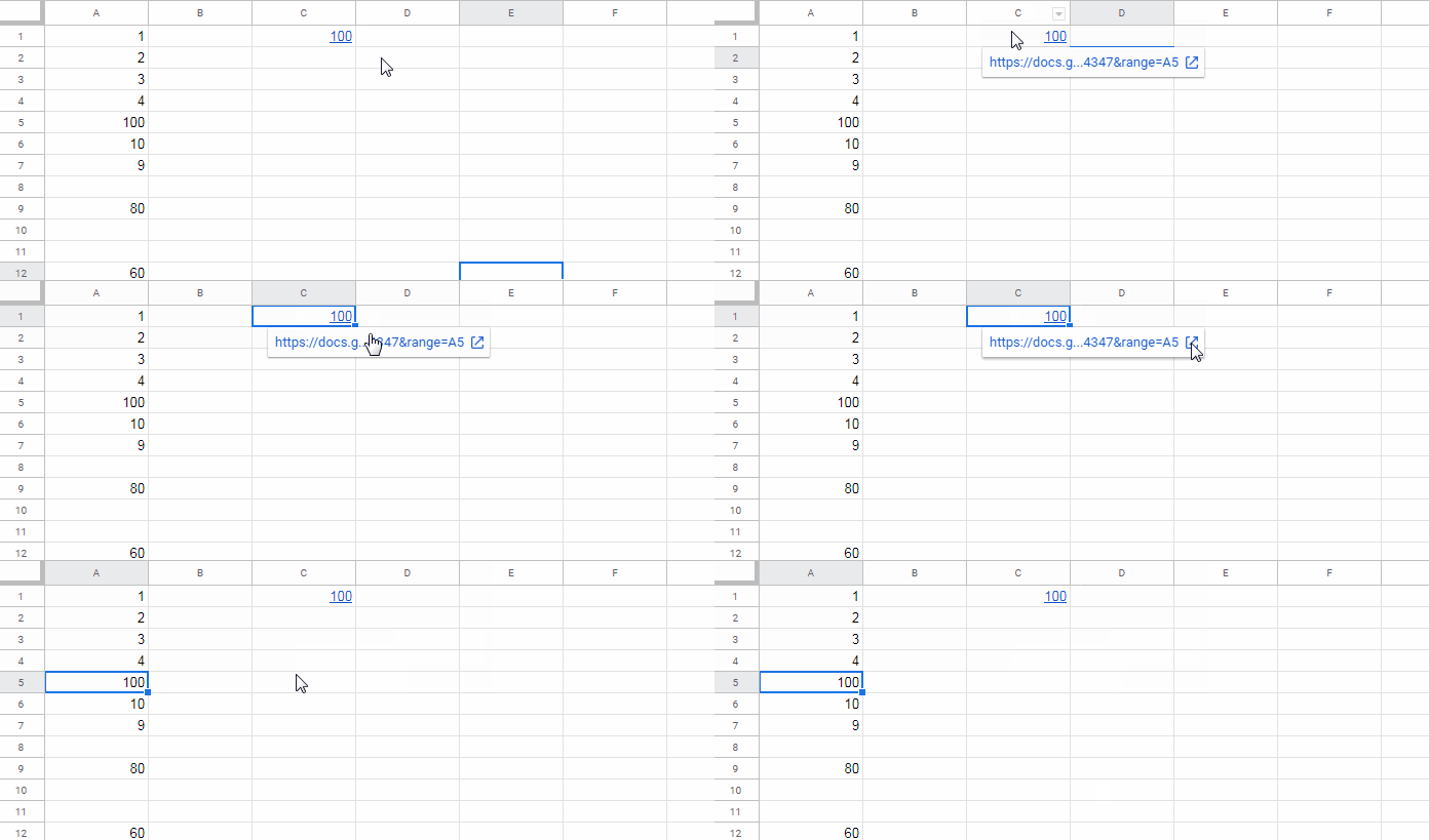
Hyperlink to Jump to Max Value Row in Google Sheets:
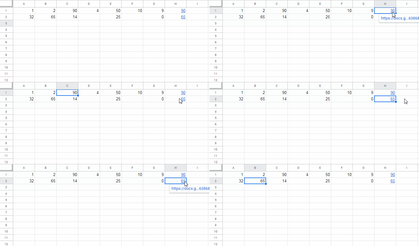
Once you have learned how to use a Hyperlink formula to jump to max value in a column or row, you can replicate the same with Min.
I haven’t seen anybody using my following techniques in Google Sheets so far. If you are interested (refer to the gif images above), continue reading.
Hyperlink Max and Min in a Column in Google Sheets
Before walking you through the formula, let me explain the formula logic. That will help you to understand the steps easily.
Hyperlink Max and Min – Formula Logic
Google Sheets is a cloud-based application. So a file created in Google Sheets has its own unique URL. I am sure, you may already know this.
The interesting thing is each cell in a Google Sheets file has its own unique URL!
For example, to get the URL of cell D10 in a Google Sheets file, right-click on cell D10 and click on ‘Get link to this cell’. Google Sheets will popup a message saying “The link copied to the Clipboard”.
The URL (link) that you have just copied can be used to hyperlink to that cell from any cell.
The URL copied from cell D10 will look like as below.
https://docs.google.com/spreadsheets/d/1Gu47Jxxxxxxxx=29xx4347&range=D10As you can see, the URL will start with the https:// protocol and ends with D10. Let me show you how to link to cell D10 from cell E1.
Seeing the syntax of the Hyperlink function will definitely help you to understand my formula.
Syntax: HYPERLINK(URL, [link_label])
How Do I Combine the URL and Link Label?
- Just replace the URL with the copied URL (already copied to the Clipboard). Do insert double quotes around it (URL).
- Replace link_label with your custom label for example “Jump” within double-quotes.
=hyperlink("https://docs.google.com/spreadsheets/d/1Gu47Jxxxxxxxx=29xx4347&range=D10","Jump")The above hyperlink formula in cell E1 will insert the hyperlink “Jump” in cell E1. Click on it (on the label “Jump”) to jump to cell D10.
Can I use this hyperlink formula in any Sheet tab?
Yes, you can!
I am coming to the key part of the logic which will help you to hyperlink to Max and Min Values in Google Sheets.
The URL is unique for all the cells within a tab, except the cell address which you can see at the end of the URL.
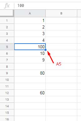
That means if we can replace D10 in the earlier copied URL with A5, clicking on the above hyperlink will take you to the cell A5.
=hyperlink("https://docs.google.com/spreadsheets/d/1Gu47Jxxxxxxxx=29xx4347&range=A5","Jump")So the key to hyperlink to max and min values in Google Sheets is finding the cell address of the max/min values.
How to Find the Cell Address of the Max and Min Values in a COLUMN in Google Sheets?
Find the cell address of Max value:
=address(match(max(A1:A),A1:A,0),1,4)Find the cell address of Min value:
=address(match(min(A1:A),A1:A,0),1,4)The above two formulas will return the cell address of the max and min values from column A. For any other column, replace A1:A with that column reference.
Formula Explanation in Short
The Match returns the row number (not relative reference) of the Min value. The Address function converts that row number to cell address.
Even if your list (min/max range) is in A10:A20, use A1:A20 or A1:A in Min. This is to find the row number, instead of relative position.
We have now all the essential elements (URL and Max/Min cell ID) to code formulas to create a hyperlink to the max as well as min value cells in a column.
Let’s see how to combine them as a formula.
Formula to Hyperlink to Max Value in Column A in Google Sheets
=hyperlink("https://docs.google.com/spreadsheets/d/1Gu47JMukHcEz4NBAxU84TTSWR_RXBxGDRkiIx2BxgPY/edit#gid=296044347&range="&address(match(max(A1:A),A1:A,0),1,4),"Max")Formula to Hyperlink to Min Value in Column A in Google Sheets
=hyperlink("https://docs.google.com/spreadsheets/d/1Gu47JMukHcEz4NBAxU84TTSWR_RXBxGDRkiIx2BxgPY/edit#gid=296044347&range="&address(match(MIN(A1:A),A1:A,0),1,4),"Min")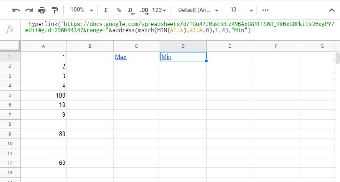
To show the max and min values itself as the hyperlink label in cell C1 and D1 respectively, replace the corresponding string in the last part of the formula with the corresponding functions.
I mean replace “Min” (including double-quotes) with min(A1:A) and similarly replace “max” (including double-quotes) with max(A1:A).
Do the Functions Large and Small Work in Hyperlink in Google Sheets?
This section answers your following queries.
- How to Hyperlink Large Value in a Column Google Sheets?
- How to Hyperlink Small Value in a Column Google Sheets?
To find the second large or second small, and then hyperlink, use the following Large/Small formulas instead of Max/Min.
=large(A1:A,2)
=small(A1:A,2)
I skip detailing this part as it’s self-explanatory. For more about these two functions and other popular Google Sheets functions, you may please go to my Function Guide.
Hyperlink Min and Max in a Row in Google Sheets
If you could understand how to hyperlink to Max and Min in a column in Google Sheets, it’s is easy to follow the below steps.
Here also the key is finding the cell address of the Min and Max, but this time in a row.
Here are those formulas.
How to Find the Cell Address of the Max and Min Values in a ROW in Google Sheets?
Google Sheets Formula to Find the Cell Address of Max in Row 1:
=address(row(A1),match(max(A1:1),A1:1,0),4)Google Sheets Formula to Find the Cell Address of Min in Row 1:
=address(row(A1),match(min(A1:1),A1:1,0),4)For row 2, use the reference A2:2 instead of A1:1.
But the issue is that I want to find the max and min, not in an entire row, but in a closed range like A1:G1. Then what changes should I make?
Simply replace A1:1 with A1:G1.
Now we can replace the cell ID in the URL with the above formulas.
Formula to Hyperlink to Max Value in Row 1 (A1:G1) in Google Sheets
=hyperlink("https://docs.google.com/spreadsheets/d/1Gu47Jxxxxxxxx=29xx4347&range="&address(row(A1),match(max(A1:G1),A1:G1,0),4),max(A1:G1))Insert the formula in cell G1 and to apply to the rows down (hyperlink to Max/Min in each row in Google Sheets) drag/copy the formula down.
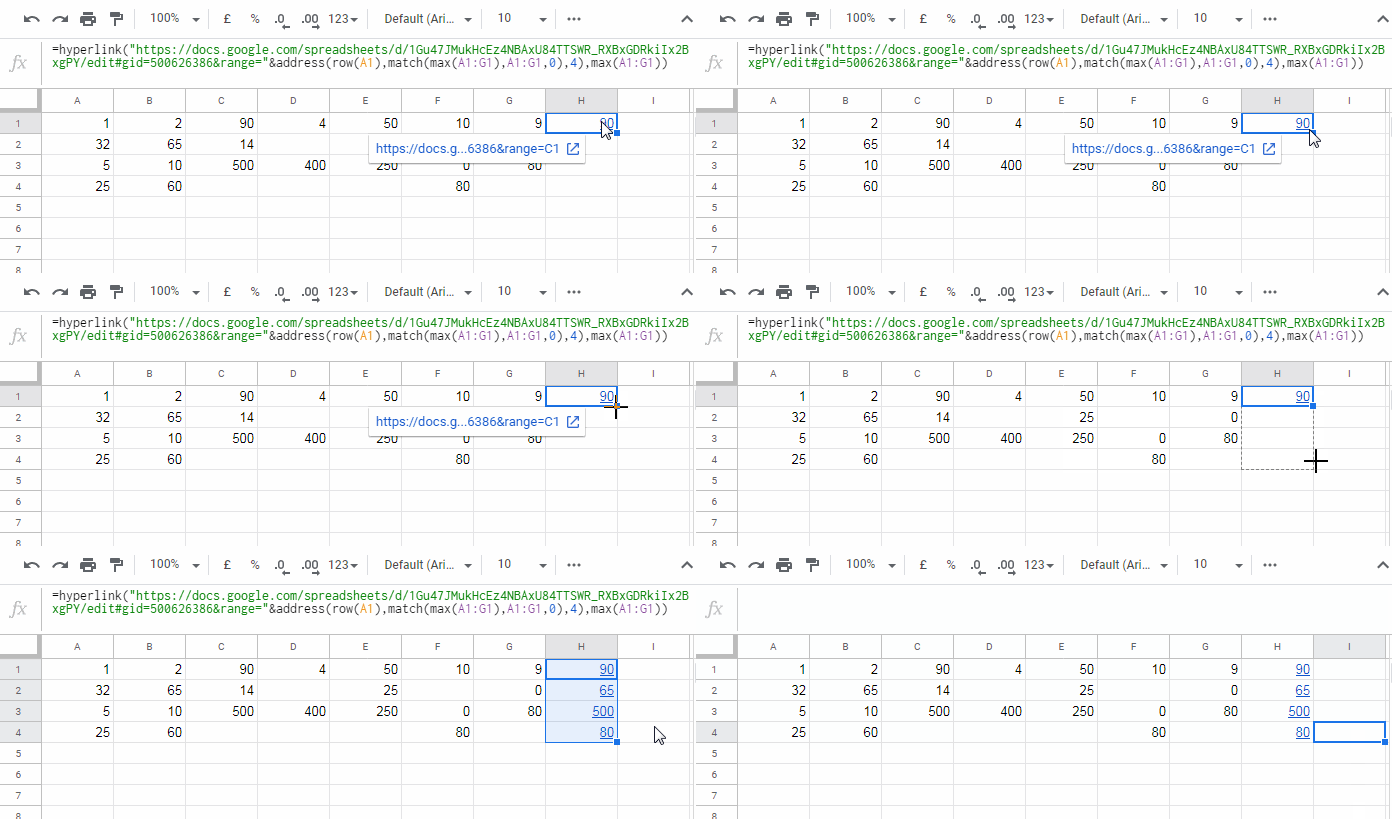
Formula to Hyperlink to Min Value in Row 1 (A1:G1) in Google Sheets
=hyperlink("https://docs.google.com/spreadsheets/d/1Gu47Jxxxxxxxx=29xx4347&range="&address(row(A1),match(min(A1:G1),A1:G1,0),4),MIN(A1:G1))Here also we can replace Min and Max with Small and Large.


