In Google Sheets, it’s possible to have different URLs behind the same link label. For example, a cell may display the label “Info Inspired,” but the actual hyperlink could be either:
https://infoinspired.com/orhttps://infoinspired.com/category/google-docs/spreadsheet/
If you apply the UNIQUE function directly to such a column, Google Sheets currently considers only the display label — not the underlying URL. As a result, it removes what appear to be duplicate entries, even when the links point to different destinations.
The Old Behavior of UNIQUE (Before 2020)
Previously, the UNIQUE function behaved differently. It used to consider the full hyperlink object — both the label and the URL — when determining uniqueness. Here’s a screenshot I captured back in 2019 that demonstrates this behavior.
The Problem with UNIQUE Duplicate Hyperlinks in Google Sheets Today
Let’s say:
- Column A contains hyperlinks with identical labels but different URLs.
- In cell B2, you apply a formula like
=UNIQUE(A2:A10).
Today, this formula will remove duplicates based solely on the label, even if the URLs differ. This change causes problems when working with datasets where the URL itself matters.
Another issue arises when you have different labels pointing to the same URL. In that case, too, UNIQUE will fail to remove what are effectively duplicate links.
So how can you correctly deduplicate hyperlinks based on their actual URLs in Google Sheets?
Solution: Use a Custom Script to Extract URLs
To properly handle UNIQUE duplicate hyperlinks in Google Sheets, we first need to extract the actual URLs behind each hyperlink.
Step 1: Add This Script to Your Sheet
- Go to Extensions > Apps Script.
- Delete any existing code and paste the following:
/**
 * Retrieves the hyperlink URL(s) from a cell or range in Google Sheets.
 *
 * @param {string} reference A single cell (e.g., "B2") or range (e.g., "B2:B10").
 * @return {string|string[][]} The URL(s) from the hyperlink(s) or an empty string if none found.
 * @customfunction
 */
function EXTRACTURL(reference) {
  try {
    const sheet = SpreadsheetApp.getActiveSpreadsheet();
    const range = sheet.getRange(reference);

    // For multiple cells, process each individually
    if (range.getNumRows() > 1 || range.getNumColumns() > 1) {
      const richTextData = range.getRichTextValues();
      return richTextData.map(row =>
        row.map(cell => {
          return cell.getLinkUrl() || "";
        })
      );
    }

    // For a single cell, return its hyperlink URL or empty string
    const url = range.getRichTextValue().getLinkUrl();
    return url || "";

  } catch (error) {
    // Log any issues and return empty string gracefully
    console.error("EXTRACTURL error:", error.message);
    return "";
  }
}- Save the script (you can name it something like
Extract URL).
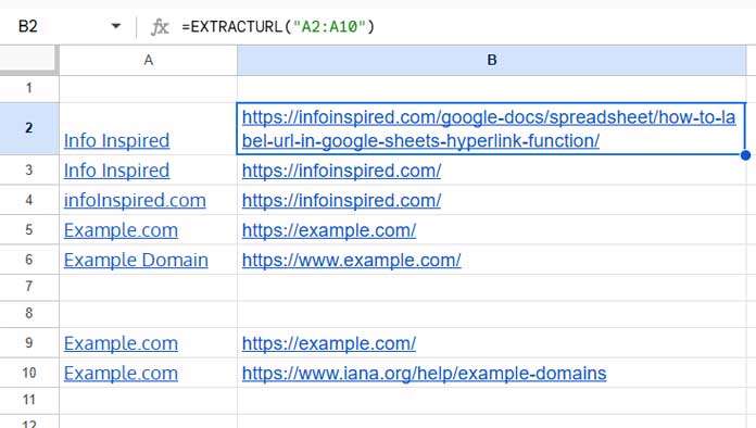
Step 2: Use the Custom Function in Your Sheet
To extract a URL from a single cell (e.g., A2), use:
=EXTRACTURL("A2")To extract URLs from a range (e.g., A2:A10), use:
=EXTRACTURL("A2:A10")This function works for hyperlinks created using the HYPERLINK function, inserted via Insert > Link, or even pasted from external sources.
Removing UNIQUE Duplicate Hyperlinks in Google Sheets — Label + URL
Once you extract the URLs into an adjacent column, you can deduplicate based on both the label and URL using the following formula:
=TOCOL(CHOOSECOLS(UNIQUE(A2:B10), 1), 1)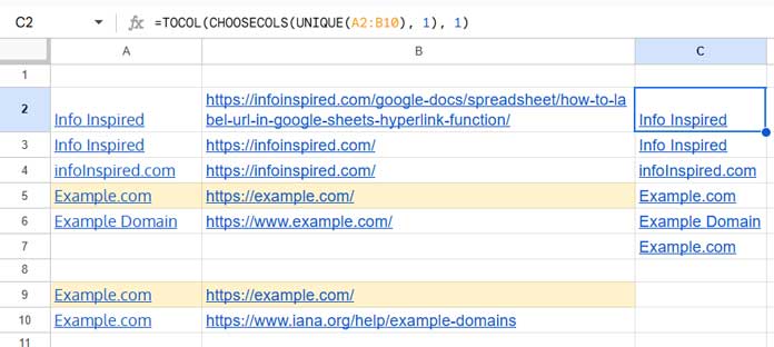
A2:B10should contain the labels in column A and the extracted URLs in column B.UNIQUEremoves duplicates only when both the label and URL match.CHOOSECOLS(..., 1)returns just the label column.TOCOL(..., 1)converts the result into a single vertical list and also removes any empty cells.
Remove Duplicates Based on URLs Only
If you want to keep only one entry per URL — regardless of the label — use this formula:
=TOCOL(CHOOSECOLS(SORTN(A2:B10, 9^9, 2, 2, 1), 1), 1)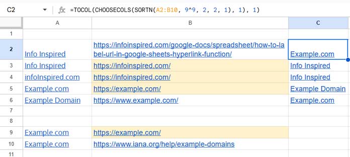
It removes duplicates based on the second column, that is the URL column. It doesn’t consider the link label. The SORTN function also sorts the result.
This works as follows:
SORTN(..., 9^9, 2, 2, 1)keeps the first occurrence of each unique URL (column 2).CHOOSECOLS(..., 1)returns the corresponding label.TOCOL(..., 1)again flattens it into a vertical list and also removes empty cells.
This approach ensures that only the first label for each unique URL is retained, solving the problem that the UNIQUE function alone cannot.
Related Resources
- Extract URLs from Hyperlinks in Google Sheets (No Scripting)
- ISURL Function in Google Sheets: Check and Validate URLs
- How to Use ENCODEURL in Google Sheets to Create Clean URLs
- XLOOKUP with HYPERLINK in Excel: Jump to Cell or URL
- Extract Usernames from Email Addresses in Google Sheets
- Create a Hyperlink to an Email Address in Google Sheets
- People Chip – Inserting and Reverting to Email Address
- ISEMAIL Function: Validate Email Addresses in Google Sheets


