In this tutorial, I’ll show you how to search for a value in Google Sheets and create a hyperlink to the found cell. This technique is useful for quickly navigating to the location of a specific value within a sheet. The search key and lookup list can be located either on the same sheet or on different sheets in the workbook.
I’ll provide a dynamic formula that works for both single-column searches and searches across multiple columns (a 2D array). The formula will remain the same in either case.
For this example, I have a Google Sheets file with two tabs: Sheet1 and Sheet2. We will search for a value in Sheet1 from Sheet2 and create a hyperlink in Sheet2 to navigate to the matching cell in Sheet1.
Two Scenarios for Searching and Hyperlinking
There are two scenarios to consider:
- Scenario 1: Search for a value in a single column and hyperlink the found cell.
- Scenario 2: Search for a value across multiple columns (2D array) and hyperlink the found cell.
Let’s explore each scenario.
Scenario 1: Search for a Value in a Single Column and Hyperlink the Found Cell
In Sheet1!A1:A10, I have a list of country names. In Sheet2!A1, I have a single country name. I want to search for this country name in Sheet1!A1:A10 and create a hyperlink to the corresponding cell in Sheet1. This will allow me to navigate from Sheet2 to the correct location in Sheet1.
Here’s the list of country names in Sheet1!A1:A10:
- Saint Vincent and the Grenadines
- San Marino
- United States
- Liechtenstein
- Eritrea
- China
- Dominica
- Philippines
- Guinea-Bissau
- Panama
In Sheet2!A1, I have the country name “San Marino.” Now, I want to create a hyperlink in Sheet2 that directs me to the cell in Sheet1 where “San Marino” is located.
Steps to Create a Hyperlink for the Found Value
Follow these steps:
- Copy the Link to the Cell in Sheet1:
- Navigate to cell A1 (or any cell) in Sheet1.
- Right-click to open the shortcut menu.
- Select View more cell actions > Get link to this cell.
- Prepare the Hyperlink Formula in Sheet2:
- In Sheet2 (cell B1), enter the following base formula to create a hyperlink:
=HYPERLINK("your_copied_Sheet1_URL_here") - Replace
"your_copied_Sheet1_URL_here"with the actual URL you copied in step #1 above. Then remove the cell reference part (A1) at the end of the URL.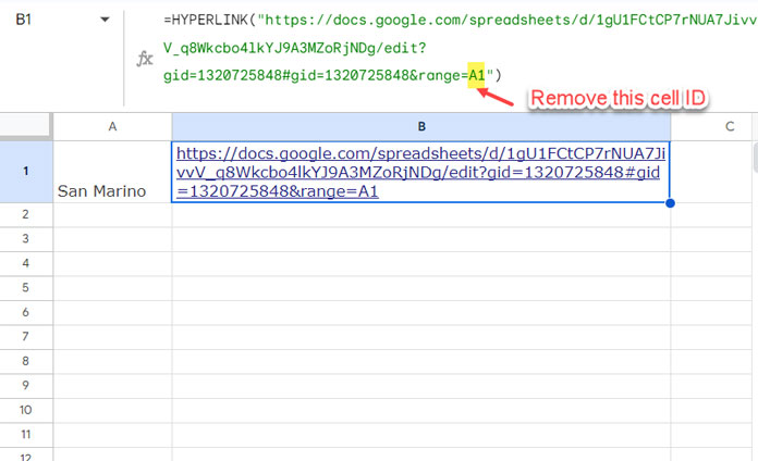
- In Sheet2 (cell B1), enter the following base formula to create a hyperlink:
- Create a Dynamic Reference for the Found Cell:
- Before the last closing bracket of the above formula, add the following dynamic formula to create a reference to the found cell:
&CHOOSECOLS(TOROW(BYCOL(Sheet1!A1:A10, LAMBDA(val, REGEXEXTRACT(SUBSTITUTE(CELL("address", XLOOKUP(A1, val, val)), "$", ""), "!(.*)"))), 3), 1) - This formula searches for the value in Sheet2!A1 within Sheet1!A1:A10 and returns the cell reference where it is found. After the above modifications, the formula should look as follows:
=HYPERLINK("https://docs.google.com/spreadsheets/d/1gU1FCtCP7rzzzzivvV_q8Wkcbo4lkYJ9A3MZoRjNDg/edit?gid=1320725848#gid=1320725848&range="&CHOOSECOLS(TOROW(BYCOL(Sheet1!A1:A10, LAMBDA(val, REGEXEXTRACT(SUBSTITUTE(CELL("address", XLOOKUP(A1, val, val)), "$", ""), "!(.*)"))), 3), 1))
- Before the last closing bracket of the above formula, add the following dynamic formula to create a reference to the found cell:
- Complete the Hyperlink Formula:
- Now, finalize the formula by adding the text label for the hyperlink. The full formula should look like this:
=HYPERLINK("https://docs.google.com/spreadsheets/d/1gU1FCtCP7rzzzzivvV_q8Wkcbo4lkYJ9A3MZoRjNDg/edit?gid=1320725848#gid=1320725848&range="&CHOOSECOLS(TOROW(BYCOL(Sheet1!A1:A10, LAMBDA(val, REGEXEXTRACT(SUBSTITUTE(CELL("address", XLOOKUP(A1, val, val)), "$", ""), "!(.*)"))), 3), 1), A1) - This formula will dynamically search for the country name in Sheet2!A1 and hyperlink it to the corresponding cell in Sheet1.
- Now, finalize the formula by adding the text label for the hyperlink. The full formula should look like this:
Result:
Clicking on the hyperlink in Sheet2 will take you directly to the matching cell in Sheet1, in this case, cell A2 where “San Marino” is located.
Scenario 2: Search for a Value Across a Range (2D Array) and Hyperlink the Found Cell
In this scenario, let’s say Sheet1 contains country names spread across multiple columns, from A1:E10. The goal is to search for a country name in this 2D array and hyperlink to the found cell.
The formula remains similar to the one in Scenario 1. The only change is that we will search across a wider range. Here’s the modified formula:
=HYPERLINK("https://docs.google.com/spreadsheets/d/1gU1FCtCP7rzzzzivvV_q8Wkcbo4lkYJ9A3MZoRjNDg/edit?gid=1320725848#gid=1320725848&range="&CHOOSECOLS(TOROW(BYCOL(Sheet1!A1:E10, LAMBDA(val, REGEXEXTRACT(SUBSTITUTE(CELL("address", XLOOKUP(A1, val, val)), "$", ""), "!(.*)"))), 3), 1), A1)In this case, replace A1:A10 with A1:E10 in the formula, allowing the search to span across multiple columns.
Formula Breakdown:
The formula is essentially a HYPERLINK formula with the following syntax:
HYPERLINK(URL, [link_label])- The link_label is the search key located in Sheet2!A1.
- The URL is the link copied from Sheet1, with the cell address removed. We dynamically add the cell reference to this URL. Here are the components of that dynamic formula:
XLOOKUP(A1, val, val): Searches for the value in Sheet2!A1 within the specified range (either a column or a 2D array in Sheet1).CELL("address", XLOOKUP(…)): Returns the absolute cell address where the value is found.SUBSTITUTE(…, "$", ""): Converts the absolute cell address to a relative reference by removing the dollar signs.REGEXEXTRACT(…, "!(.*)"): Removes the sheet name from the cell address, leaving only the cell reference.BYCOL(Sheet1!A1:A10, …): The BYCOL function applies the above LAMBDA function to each column in the specified array (which can be a single column or multiple columns).TOROW(…): Removes errors from the results.CHOOSECOLS(…): Selects the first found cell in the range, ensuring you receive the correct hyperlink even when searching within a 2D array.
That’s it! You’ve successfully learned how to search for a value and hyperlink the found cell in Google Sheets. This technique works for both single-column searches and searches across multiple columns, making navigation in large sheets much easier.
Resources
- Create a Hyperlink to the Vlookup Output Cell in Google Sheets
- Extract URLs from Hyperlinks in Google Sheets (No Scripting)
- UNIQUE Duplicate Hyperlinks in Google Sheets – Same Labels Different URLs
- How to Create a Hyperlink to an Email Address in Google Sheets
- Hyperlink Max and Min Values in Column or Row in Google Sheets
- Hyperlink to Index-Match Output in Google Sheets
- Inserting Multiple Hyperlinks within a Cell in Google Sheets
- Hyperlink to Jump to Current Date Cell in Google Sheets
- Jump to the Last Cell with Data in a Column in Google Sheets (Hyperlink)
- Hyperlink Calendar Dates to Events in Google Sheets
- Using HYPERLINK with FILTER Function in Google Sheets


Hi Prashanth, perfect, it was very fast. Thanks a lot for your help. It works very well. Regards.
Hi, It works well!
Is it possible to hyperlink matched value by the functions INDEX/MATCH instead of the VLOOKUP?
Thanks.
Yes! I will update you with a tutorial soon.
Hi, Roman,
It’s ready now!
Hyperlink to Index-Match Output in Google Sheets.
Cheers!