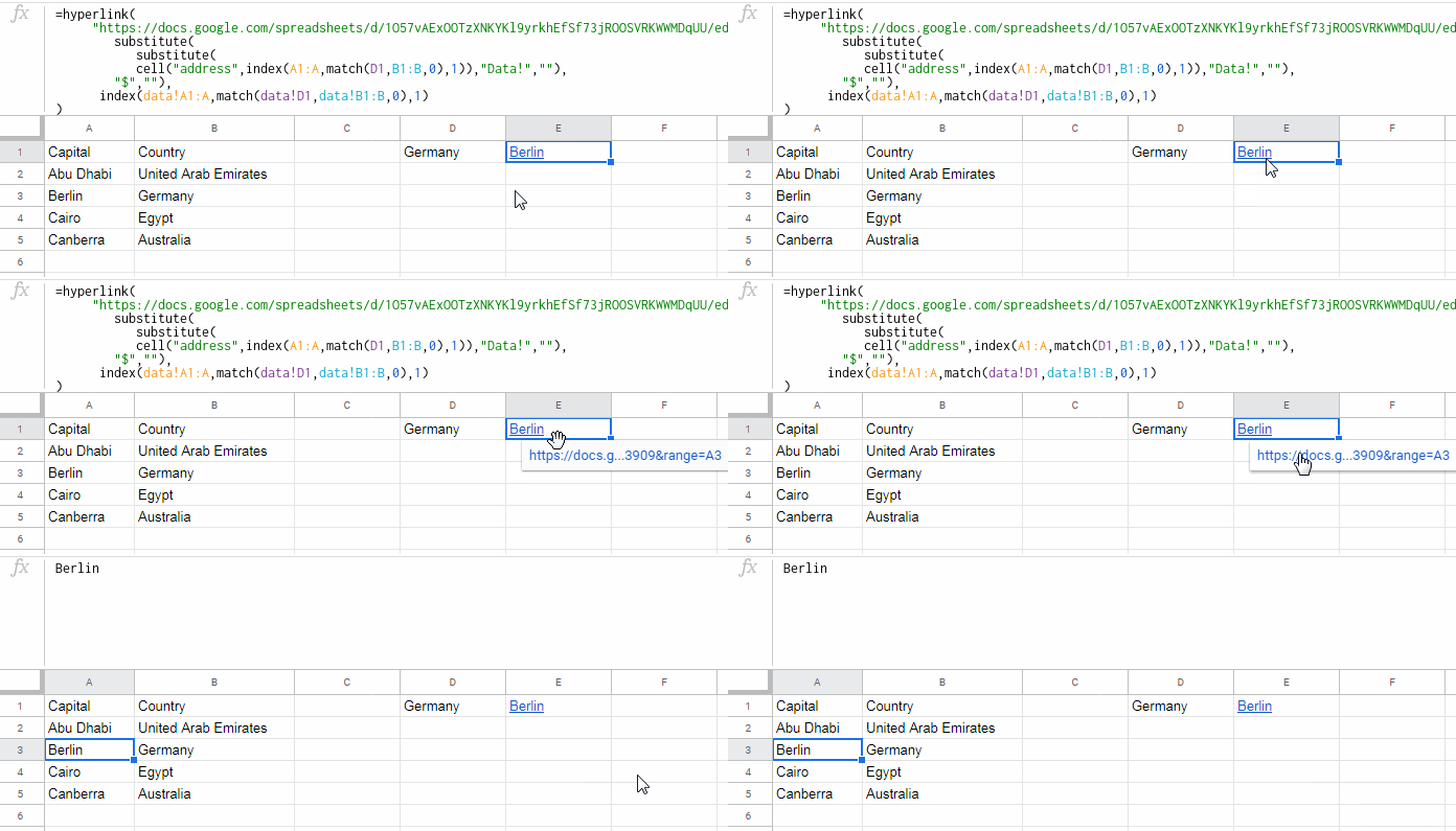
Google Sheets supports creating a hyperlink to an Index-Match output cell. The output thus returned (Index-Match value) will be a clickable link (hyperlink) in Google Sheets.
Please do note one thing. The row/column argument in Index should not be 0 as it causes multiple values in the output.
In short, as per my tutorial, you can only hyperlink to a single cell output of Index-Match in Google Sheets.
Introduction to Hyperlink Index and Match in Google Sheets
Index-Match is a popular alternative among Excel users for Reverse Vlookup. But it now seems replaced by a new function called XLOOKUP.
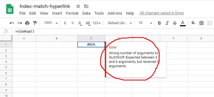
As far as I know, there is no XLOOKUP function so far in Google Sheets. I guess Google will include this function soon (I may be wrong)!
The below picture says why I think so.

In Google Sheets, for reverse Vlookup, it doesn’t require the XLOOKUP as Vlookup itself is capable of that.
You May Like: Reverse Vlookup Examples in Google Sheets [Formula Options].
Even though it’s not a must to use Index-Match, many Google Sheets users, who are well conversed in Excel, prefer to use Index-Match.
So in this post let’s learn how to hyperlink Index-Match result in Google Sheets. It makes sense, right?
Here I’m following the same approach that I have used in hyperlinking to Vlookup output cell in Google Sheets. Just I’m replacing Vlookup in that approach with Index-Match here.
How to Hyperlink to Index-Match Result in Google Sheets
I am using a very simple table so that you can easily create it for the testing of my formula. It contains the names of a few countries and their national capitals.
| National Capital | Country Names |
| Abu Dhabi | United Arab Emirates |
| Berlin | Germany |
| Cairo | Egypt |
| Canberra | Australia |
Create the above table in the range A1:B5 and rename the sheet as ‘data’. Then follow the below steps to create a hyperlink to Index-Match output cell in Google Sheets.
Index-Match Formula (for Hyperlinking)
I know you are already using Index-Match. Still, I’m explaining the use to make this tutorial beginner-friendly.
Example:
I want to match “Germany” in the above table in column B, then offset that much number of rows in column A and get the value “Berlin”.
To match the country (string) “Germany” in column B we can use the MATCH function by following this syntax – MATCH(search_key, range, search_type).
Key the search_key “Germany” in cell D1 and use this Match formula in cell E1. The formula would return 3.
=match(D1,B1:B,0)That means we want to offset 3 rows in another column, here column A and fetch the value “Berlin”. How?
We can use the INDEX function as per the syntax – INDEX(reference, row, column).
=INDEX(A1:A, 3, 1)Simply replace the # 3 with the Match formula itself. Here is that Index-Match formula to return the “Capital” of the “Country” Germany.
=index(Data!A1:A,match(Data!D1,Data!B1:B,0),1)
Note:
The # 1 in the formula represents the column number to offset. The Index ‘reference’ is A1:A, which means column 1.
If the ‘reference’ is A1:E and you put 5 as column number, then the formula would offset 3 rows in column E.
Now let’s see how to hyperlink to this index-match output/result in Google Sheets or we can say make the label “Berlin” in cell E1 clickable.
Hyperlinking Techniques
There are actually 3 steps involved in hyperlinking an Index-Match result in Google Sheets. We have already completed step 1 in that! Here are those 3 steps.
- Index-Match formula (we will hyperlink the output of this formula): ✓
- URL of the cell A1 from the ‘data’ sheet. Here my sample table is in the sheet named ‘data’: ✘
- Cell ID of the Index-Match formula output: ✘
Only the steps 2 and 3 are pending.
Step 1
=index(Data!A1:A,match(Data!D1,Data!B1:B,0),1)Step 2
To get the URL, right-click on cell A1 in the ‘data’ sheet and click “Get link to this cell”.
Right-click and paste the copied link in cell E2. After pasting, edit the link to remove the cell reference A1 at the end of the link.
https://docs.google.com/spreadsheets/d/****#gid=92***9&range=The above URL is a sample. You must use the link copied from your sheet as above. The = sign must be the last character after editing the link as mentioned above.
Step 3
In cell E3, use the step 1 Index-Match formula within the CELL function to get the cell ID of the Index-Match output.
Please follow the below Generic Formula for getting the cell ID of the Index-match result value.
=cell("address",index-match_formula)Formula:
=cell("address",index(Data!A1:A,match(Data!D1,Data!B1:B,0),1))The above formula would return the cell address $A$3. We must clean it by removing the $ sign from the formula.
Also if your table is ‘data’ sheet and the formula is in another sheet in that file, then the result would be data!$A$3.
So whether the sheet name is there or not with the cell address, let’s include the provision to remove the string data! from the result.
Just modify the formula in cell E3 to include multiple Substitute functions as below.
=substitute(
           substitute(
           cell("address",index(A1:A,match(D1,B1:B,0),1)),"data!",""),
        "$","")
The first Substitute removes the $ sign whereas the second one removes the data! sub-string if any. The result of the above formula will be the cell ID ‘A3’.
Using Step 1, 2, and 3 Formulas within Hyperlink to Create Hyperlink to Index-Match Result
The Hyperlink function takes two arguments. They are ‘URL’ and ‘link_label’.
Syntax: HYPERLINK(URL, [link_label])We can use the Index-Match formula (step 1) as the ‘link_label’ in Hyperlink. What about ‘URL’?
The ‘URL’ must be the combined output of step 2 and step 3 formulas. The following Generic formula will help you understand this.
=hyperlink(
     "step_2"&
        step_3,
      step_1
)
Formula that Hyperlinks Index-Match Output (based on the Generic Formula above):
=hyperlink(
     "https://docs.google.com/spreadsheets/d/****#gid=92***9&range="&
        substitute(
           substitute(
           cell("address",index(A1:A,match(D1,B1:B,0),1)),"Data!",""),
        "$",""),
      index(data!A1:A,match(data!D1,data!B1:B,0),1)
)
Now remove formulas in the cell E1, E2, and E3. Insert our above final formula in cell E1 and voila!

Resources:
- How to Label URL in Google Sheets Using HYPERLINK Function.
- Search Value and Hyperlink Cell Found in Google Sheets.
- UNIQUE Duplicate Hyperlinks in Google Sheets – Same Labels Different URLs.
- Hyperlink Max and Min Values in Column or Row in Google Sheets.
- Case Sensitive Reverse Vlookup Using Index Match in Google Sheets.
- Multiple Conditions in Index Match in Google Sheets.


Can I index match from another google sheet and do the same functions?
Hi, Midhun,
It’s not possible. But there is a workaround that I will post soon! Please stay tuned for my upcoming post.
Could you show a file with an example? Thank you!!
Hi, Mario,
Thanks for letting me know. Added the link button at the end of the post.