One of the best examples of combination formulas is Index and Match. It’s popular in spreadsheet applications like Excel and Google Sheets for vertical lookup. You can use multiple conditions in Index Match in Google Sheets.
Many people are addicted to Index Match, and even if they can use Vlookup, they use Index and Match combo. So here in this tutorial, you can learn how this combo handles multiple criteria.
Multiple Conditions in Index Match in Google Sheets
Here is an example of the use of more than one condition in Index Match.

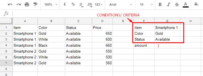
Here in this example, I have two smartphone products in Colum A. Each smartphone has three variants based on color.
The multiple conditions to use in Index Match are marked in the screenshot. From that, you can understand that I want to look up the price of Smartphone 1 of which the “Color” is “Gold” and “Status” is “Available”.
The item is in row # 2, and the price is $ 650.00.
Here we want the formula to lookup three conditions. So how can we use that?
Index Match Formula to Lookup Multiple Conditions
Here is the formula to lookup multiple conditions in Index Match in Google Sheets.
Master Index Match Formula
This is the formula that you can use in cell G4 in the above example.
=ArrayFormula(index(A2:D,match(concatenate(G1:G3),A2:A&B2:B&C2:C,0),4))I think I can explain this formula in a way that you can easily follow.
The Match Formula Part
In this section, I am going to detail to you how the Match formula in the above formula works.
Note:- Switch to the Tutorial on the use of Match Function in Google Sheets.
Syntax:
MATCH(search_key, range, [search_type])Step 1:
Combine the conditions to use as search_key in the Match.
=concatenate(G1:G3)It will return the below string which is the search key in the Match function.
Result: Smartphone 1GoldAvailable
Step 2:
Now to the range in Match (you won’t see the ArrayFormula in the master formula with it as it’s moved to the front).
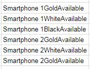
=ArrayFormula(A2:A7&B2:B7&C2:C7)This formula returns the below one-column values.

The Match formula in the Master Index Match formula above looks for the search key “Smartphone 1GoldAvailable” (Step 1 output) in the Step 2 output and returns # 1 as the relative position since the search key can be found in the first row of Step 2 output.
The above two steps are the key to performing multiple conditions in the Index Match formula in Google Sheets.
The Index Formula Part:
Syntax:
INDEX(reference, [row], [column])In this, the reference is our 4 columns original data range A2:D and the Row is the # 1 returned by the Match formula above.
We want the Index formula to return the Price, which is in column 4.
So the abbreviated version of our Master Index Match formula is as below.
=ArrayFormula(index(A2:D,1,4))In this, replace 1 (row) with the Match formula.
That’s all. I hope you can learn how to use multiple conditions in Index Match in Google Sheets.
Conclusion
You can use Vlookup too in this case. Here is that formula!
=ArrayFormula(vlookup(CONCATENATE(G1:G3),{A2:A10&B2:B10&C2:C10,D2:D10},2,false))Similar to multiple criteria in Index Match, you can combine the conditions here to use in Vlookup.
Here the range part is a little different. Here instead of A2:D in Index Match, I’ve used a virtual range with two columns. The first three columns are combined into one and then added the Price column. So the Vlookup Index column is 2 here.
Honestly, the above two are not the best solutions. We can solve the same problem with an easy-to-read FILTER. Here you go!
=filter(D2:D7,A2:A7=G1,B2:B7=G2,C2:C7=G3)Thanks for the stay. Enjoy!
Related Reading:


Hello Prashanth,
Your website is incredible. Thank you so much. It is a fantastic tool for learning Google Sheets.
My question is,
I have a very messy sheet used for scheduling. I want to find a client that could be anywhere in multiple columns.
In a new sheet, create a formula to search for a specific client and then return data associated with that client, such as cost, time, or income.
Is this possible to do with functions?
– URL (sample sheet) removed by admin –
Hi, Jack Christmann,
I’ve sent my request to get edit access to your sheet.
Further, in that sheet, show me your expected result.
That’ll possibly help me to understand the problem.
Thank you, Prashanth,
I granted you to access and expanded on what I was looking for in yellow.
I have tried messing around with different formulas to try to get the result I am looking for but have constantly failed.
I am wondering if what I am trying to do is even possible, or perhaps I need to change the way I have my data setup.
Thanks!
Hi, Jack Christmann,
Please check your sheet for my formula and a short note.
Can you provide more images and diagrams for this article? Seeing the code with the example spreadsheet is the most helpful for me.
Hi, Emily Stroud,
Based on your request I have updated the post to included a sample sheet.