This post explains how to use the INDEX MATCH to find the minimum, maximum, or specific value in every nth column in Google Sheets and return a corresponding value.

The formula can be somewhat complex because of the involvement of the nth parameter. However, the LET function can be used to make it easier to understand.

As a side note, INDEX and MATCH are two independent functions, but we are talking about their combined use. The scenario is as follows.

Sometimes we keep every other or nth column in a table for specific purposes, such as inputting totals of the columns to the left.

How do we look up a value (search_key) in those columns and return a value from a corresponding column in a different row?

For example, I want to find the minimum value in every fourth column in a row and return the corresponding value from the same column in another row.

In the following table, I have the quarterly production quantities of an item in columns E, I, M, and Q.

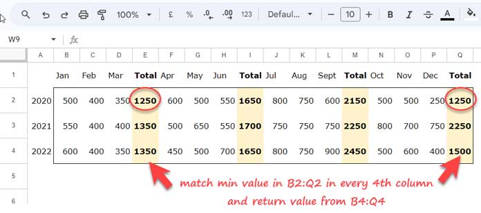
I want to use the INDEX MATCH function to find the minimum production in every fourth column (every quarter) in row 2 (the year 2020) and return the corresponding quarter’s production in row 4 (the year 2022).

We typically use the MATCH function to match a value and the INDEX function to offset that result.

In the first example, we will see how to use the INDEX MATCH combo to find the minimum value in every nth column in Google Sheets and return the corresponding value in another row.

If there are multiple matching values, we will use the FILTER function instead to return all of them.

Once you have learned this technique, you can apply it to INDEX MATCH a maximum value or any other specific value in Google Sheets.

INDEX MATCH Minimum Value in Every Nth Column in Google Sheets

We will use the above table for the example. Here is the formula:

=ARRAYFORMULA(
     LET(
          f_row,B2:Q2,
          r_row,B4:Q4,
          n,4,
          test,MOD(SEQUENCE(1,COLUMNS(f_row)),n),
          fnl,IF(test=0,f_row,),
          INDEX(r_row,1,MATCH(MIN(fnl),fnl,0))
     )
)

where;

• f_row (find row): The range of cells in row 2 (B2:Q2) that contains the values to match.
• r_row (return row): The range of cells in row 4 (B4:Q4) that contains the values to return.
• n: The number of columns to skip between each match. To find the minimum value in every other column set n to 2.

We will see the rest of the formula parts, namely test, fnl, and the INDEX MATCH every nth column formula in the anatomy section below.

However, when you use the formula to INDEX MATCH the minimum value in every nth column, you only need to modify the above three arguments. Specifically, you should replace:

• B2:Q2 with the row that contains the values to match.
• B4:Q4 with the row that contains the values to return.
• 4 with the number of columns to skip between each match.

Please note that f_row and r_row must be of equal size.

Anatomy of the Formula

The following MOD-based formula returns 0 in every fourth column.

=ARRAYFORMULA(MOD(SEQUENCE(1, COLUMNS(B2:Q2)), 4))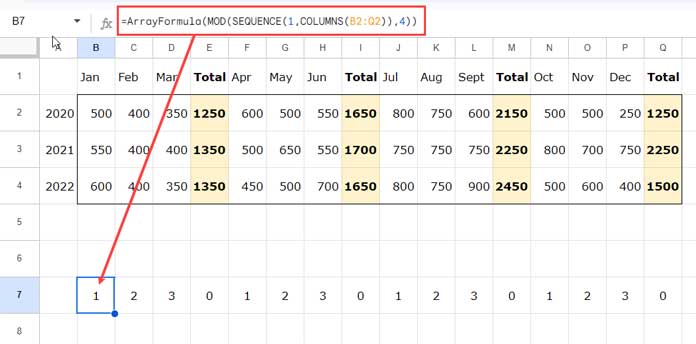

In our master formula, the relevant part is MOD(SEQUENCE(1, COLUMNS(f_row)), n).

The name given to this value expression is test.

Next, we have used an IF logical test to return B2:Q2 if the test range is equal to 0 (zero), or else an empty string.

=ARRAYFORMULA(IF(B7:Q7 = 0, B2:Q2, ""))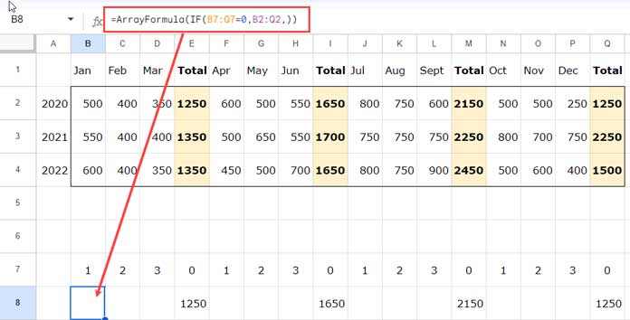

In our master formula, the relevant part is IF(test = 0, f_row, "").

The name given to this value expression is fnl.

Now what is left is the INDEX MATCH every nth column formula.

=INDEX(B4:Q4,1,MATCH(MIN(B8:Q8),B8:Q8,0))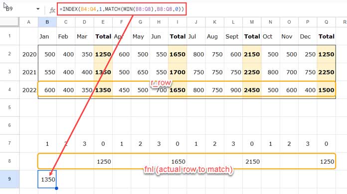

Here is the relevant part in the master formula:

INDEX(r_row, 1, MATCH(MIN(fnl), fnl, 0))

INDEX MATCH Maximum Value in Every Nth Column in Google Sheets

As per our sample data in the previous example, here is the formula to INDEX MATCH the maximum value in every nth (4th) column in Google Sheets.

=ARRAYFORMULA(
     LET(
          f_row,B2:Q2,
          r_row,B4:Q4,
          n,4,
          test,MOD(SEQUENCE(1,COLUMNS(f_row)),n),
          fnl,IF(test=0,f_row,),
          INDEX(r_row,1,MATCH(MAX(fnl),fnl,0))
     )
)

It’s the same formula with one key difference. Here we have used the MAX function instead of MIN.

How to Handle Multiple Matching Values in Every Nth Column in Google Sheets

The above formulas have one common issue: they cannot return multiple values.

In the above first formula example, 1250 is the minimum value in the range B2:Q2. It appears in cells E2 and Q2. So the results from the corresponding columns from the range B4:Q4 must be 1350 and 1500.

However, the INDEX MATCH minimum value formula only returns 1350.

This is one of the drawbacks of this combination. We can solve this by using the FILTER function.

In the formula, replace the INDEX(r_row,1,MATCH(MIN(fnl),fnl,0)) with FILTER(r_row,fnl=MIN(fnl)).

So the formula will be:

=ARRAYFORMULA(
     LET(
          f_row,B2:Q2,
          r_row,B4:Q4,
          n,4,
          test,MOD(SEQUENCE(1,COLUMNS(f_row)),n),
          fnl,IF(test=0,f_row,),
          FILTER(r_row,fnl=MIN(fnl))
     )
)

You may replace MIN within the FILTER with MAX to match the maximum value in every 4th column in the range B2:Q2 and return the corresponding values from the range B4:Q4.

INDEX MATCH Every Nth Column with Specific Criteria

In all of the above examples, we have matched the minimum or maximum value in the range B2:Q2. However, it is not necessary to restrict ourselves to minimum and maximum values. We can use any condition, even a text criterion.

Here is a different example, where I want to find whether an employee was present (represented by the letter P) on any Sunday and, if so, the corresponding date.

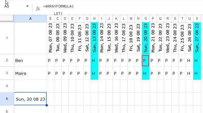
Here, the range to match is B2:V2 (referred to as f_row), the offset range is B1:V1 (referred to as r_row), and n is 7. In addition to that, we should replace MAX(fnl) or MIN(fnl) with the text value "P".

=ARRAYFORMULA(
     LET(
          f_row,B2:V2,
          r_row,B1:V1,
          n,7,
          test,MOD(SEQUENCE(1,COLUMNS(f_row)),n),
          fnl,IF(test=0,f_row,),
          INDEX(r_row,1,MATCH("P",fnl,0))
     )
)

To INDEX MATCH every nth column and return multiple values, you may replace the INDEX(r_row, 1, MATCH("P", fnl, 0)) formula with the following FILTER(r_row, fnl = "P") formula.

Conclusion

I intentionally kept quiet about one important aspect of the INDEX MATCH every nth-column formula. It’s about the nth.

For example, if nth is 4, how do we start nth from the first column in the range instead of the fourth column?

I mean, instead of 4, 8, 12, 16, 20, how do we use 1, 5, 9, 13, 17? What changes shall we make in the formula?

Please modify the MOD(SEQUENCE(1, COLUMNS(f_row)), n) formula. You may replace it with MOD(SEQUENCE(1, COLUMNS(f_row), n), n).