MOD is a mathematical function in Google Sheets. You can learn here the purpose of this function and also how to use the MOD mathematical function in Google Sheets. Please don’t confuse it with MODE, which is a statistical function.

The purpose of the MOD Mathematical function in Google Sheets is to return the remainder after a division.

Syntax:

MOD(dividend, divisor)

Dividend: The number that you want to divide to find the remainder.

Divisor: The number by which you want to divide the Dividend.

Examples of the Use of MOD Mathematical Function in Google Sheets

Here are few examples to learn the use of Google Sheets MOD formula.

Formula: =MOD(6,4)
Result: 2

See one more example.

Formula: =MOD(9,3)
Result: 0

Still, have doubt using MOD in Google Doc Spreadsheets? See few more examples.

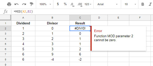
In this example, you can see that the MOD formula in cell C2 returns an error as the divisor can’t be zero in MOD.

Then in row # 8, the MOD formula returns negative value as the divisor is negative.

What’s the Real Life Use of Google Sheets MOD Mathematical function?

To answer this question, honestly, I don’t have much in my armoury. I think I used this function only once or twice in the past. But I can give you a clue on how to use MOD formula in real life situations.

Some functions in Google Sheets accept other functions as function arguments and MOD is no exception. So I have one example for you that you can dynamically use to form complex formulas.

As a side note, if you ask me to name one function that does not accept other formulas as arguments in it, I would say SUBTOTAL.

In my testing, it didn’t accept other functions as its arguments. It may vary in Excel and Google Sheets.

For example, the SUMIF function in Google Sheets supports ROW function as one of its arguments while in Excel it’s not so.

See my running total formula in Google Sheets where I’ve used ROW function in SUMIF as an argument. If you try this in Excel, it may not work!

Now back to our tutorial about Google Sheets MOD function. Here is one example formula that you can use to form complex formulas involving Google Sheets MOD function.

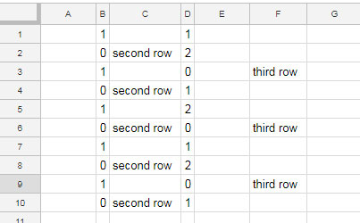
In the above example, I’ve two formulas. One in cell B1 and another in cell D1. See those formulas below.

The formula in B1.

=ArrayFormula(MOD(ROW(A1:A10),2))

The formula in D1.

=ArrayFormula(MOD(ROW(A1:A10),3))

Both these formulas are array formulas involving MOD and ROW functions. What they return you can see in the screenshot.

This piece of formulas you can use to form complex other useful formulas. For example, you can filter column D for the value 0 using Filter or Query. That means you can either filtered out or extract the values in every third row.

That’s all. Hope you find this tutorial useful. Enjoy!