Extract URLs from Hyperlinks in Google Sheets (No Scripting)

Extracting hyperlinks or embedded URLs in Google Sheets is possible without relying on Google Apps Script (GAS).

It doesn’t matter whether the links are (1) formula-based links or (2) embedded links, the method will work flawlessly.

You can refer to the two types of links in Google Sheets as:

Formula-Based Links: Created using the HYPERLINK function. For example: =HYPERLINK("https://infoinspired.com/", "InfoInspired"). These are explicitly defined in the cell formula and show the URL when using FORMULATEXT.
Embedded Links: You insert these links using the Insert > Link menu option. These links embed in the cell or text and do not reveal the URL when using FORMULATEXT.

For example, if cell A1 contains a link, =FORMULATEXT(A1) will return the cell formula if it contains a formula-based link. If it doesn’t contain a formula, it will return #N/A.

Extract URLs from Hyperlinks Individually (Built-in Method)

This method allows you to copy a URL from a link in a cell, regardless of whether the link is formula-based or embedded.

Steps:

Hover your mouse pointer over the link.
A small box will appear with options to copy, edit, and delete the hyperlink.
Click on the copy-link icon.
Right-click any cell and select Paste.

How to Extract URLs from Hyperlinks in a Column (Workaround)

Extract URLs from Hyperlinks or Embedded Links in a Column

The built-in method is impractical if multiple links are in a column, as copying the URLs individually is time-consuming.

Instead, we will use a workaround that you can easily perform in a few steps without needing knowledge of Google Apps Script.

This method also applies to both formula-based hyperlinks and embedded links.

For example, we’ll consider the range A2:A5 in the tab named “Sheet1” and extract the URLs into B2:B5 in that sheet.

Step 1: Publish the Tab “Sheet1”

In this step, we will publish the sheet on the web. By doing this, Google converts the spreadsheet data into an HTML format, hosts it on its servers, and provides a URL for access.

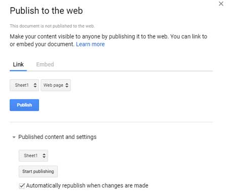
Go to the File menu, click on Share, and select Publish to web. Be cautious about publishing sensitive data, as anyone with the link can view the published content. However, you can unpublish it at any time.
Under Link, select the tab name (i.e., “Sheet1”) in the first drop-down and then select web page in the second drop-down.
Click Publish.
Once published, you will get a link URL. Copy that.

Step 2: Import Published Google Sheets Contents Back to Google Sheets

In cell A1 in “Sheet2” of the same Google Sheets file, right-click and paste the copied URL.
In cell B1 in “Sheet2”, enter the following formula and wait for it to return a list of all the href values (URLs) found within anchor tags in the given HTML document:

=IMPORTXML(D1, "//a/@href")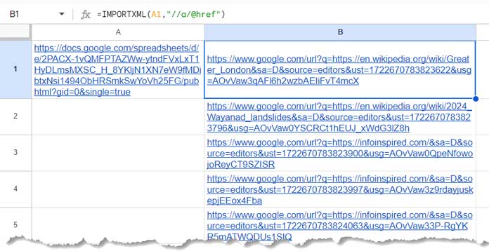

IMPORTXML formula extracts URLs from website links

Step 3: Extracting URLs

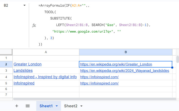
In cell B2 of “Sheet1”, enter the following formula and voila!

=ArrayFormula(IF(A2:A="",,
   TOCOL(
      SUBSTITUTE(
         LEFT(Sheet2!B1:B, SEARCH("&sa", Sheet2!B1:B)-1), 
       "https://www.google.com/url?q=", ""
   ), 3)
)

Formula Explanation:

The LEFT function extracts n characters from the left of the strings in Sheet2!B1:B, where n is determined by the SEARCH formula: SEARCH("&sa", Sheet2!B1:B)-1.
The SUBSTITUTE function replaces “https://www.google.com/url?q=” in the values extracted by the LEFT function with “”.
The TOCOL function removes errors and empty strings from the output.
The IF function removes values in the TOCOL output if the corresponding rows in A2:A are blank.

That’s how we can extract multiple URLs from hyperlinks in Google Sheets.

Resources

15 COMMENTS

Kevin Michael Valenzuela March 2, 2021 At 6:05 am

You’re the best at this bro. Sending love from the Philippines.

sib October 14, 2020 At 6:51 pm

Thanks !

Jessa Mae Deloy August 6, 2020 At 8:54 am

This is really helpful! Thank you, Prashanth.

bahar May 21, 2020 At 5:55 pm

Hi Prashanth,

I was looking to get the ‘Sheet3’ url into a cell A1 with only formula (without script).

Thank You.

- Prashanth May 23, 2020 At 7:57 am
  
  Hi, Bahar,
  
  I don’t find any supporting function in Google Sheets.
  
  As you may know, manually we can do that with right-clicking on Sheet3!A1 and click “Get link to this cell”.
  
  - bahar May 23, 2020 At 12:28 pm
    
    Hi Prashanth,
    
    Thank you for your response, have a great day.
    
    Thank You.
    
Wayne May 11, 2020 At 9:17 pm

This worked, thank you!

(Note: It does not work if you’re signed in to your company’s Gsuite account. Make sure to sign in to your personal Google account before starting the steps).

- Prashanth May 12, 2020 At 8:44 am
  
  Hi, Wayne,
  
  Thank you for your valuable feedback.
  
- Misha October 22, 2020 At 11:14 am
  
  Is there a way to get this to work without unrestricted publishing (i.e., within a company G-Suite account)?
  
Hamza August 20, 2019 At 6:38 pm

Thanks man really helpful

Ben August 13, 2019 At 11:03 pm

Amazing – Thank you for sharing!

Pat M February 14, 2019 At 4:03 am

Prashanth,

So, I tried a couple of different things. The sheet I was trying to copy had around 1900 rows of URLs.

Seems like the largest number of rows it will work with is around 1000

To get it to work, I had to break it up into two sheets and just run the process twice.

Pat

- Prashanth February 14, 2019 At 7:27 am
  
  Hi,
  
  I think that’s the case.
  
  There are similar issues with all the text functions like, join, textjoin, ampersand sign, concatenate etc.
  
  Best,
  
Pat M February 13, 2019 At 12:21 am

Prashanth,

I did everything as outlined above for Google Sheets. When I went to Step 3 it returned the following Error.

“Resource at URL Contents Exceeded Maximum Size”

Thoughts?

Pat

- Prashanth February 13, 2019 At 8:12 am
  
  Hi, Pat,
  
  Actually, I was unaware of that issue due to my testing with a limited dataset.
  
  Thanks for the info.
  
  You can try the following workaround.
  
  Remove unwanted rows and columns in your Sheet (published). The aim is to reduce the file size. Then try.
  
  If that doesn’t work, try to import a limited number of rows.
  
  Existing Formula.
  
  =IMPORTXML("URL","//a/@href")
  
  Play around with;
  
  =Array_Constrain(IMPORTXML("URL","//a/@href"),500,1)
  
  This formula imports 500 rows and 1 column.
  
  But I didn’t test any of the above workarounds.
  
  Thanks for your understanding.
  
  Best