In this blog post, we will show you how to use the HYPERLINK function to link calendar dates to events in Google Sheets. This will be very helpful for organizing your events and improving your workflow.

We will walk you through the process of creating an interactive calendar template that dynamically responds to month selections and year changes, and establishes links between dates and events in a separate sheet.

I’ve previously shared a dynamic yearly calendar template for use in Google Sheets, which utilizes formulas for each week. However, in this tutorial, we’ll focus on individual formulas for each date, enabling us to hyperlink calendar dates to specific events.

Let’s get started by creating an interactive calendar, and then we’ll move on to hyperlinking the dates. But first, here’s my pre-built template with all the necessary formulas.

Calendar Preview and Download

Creating an Interactive Calendar in Google Sheets

To hyperlink dates to events, we require two sheets within a file: an interactive calendar that responds to month selection in a drop-down, and a sheet with dates in one column and events in another column.

Let’s start by creating the interactive calendar in Google Sheets.

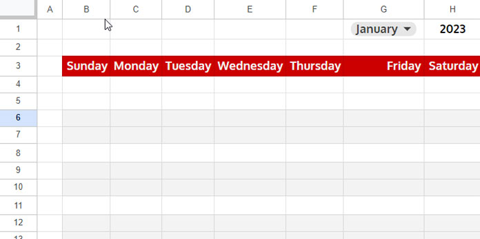
Creating the Layout of the Interactive Calendar

1. Go to https://sheets.new/ to create a Google Sheets file with a blank spreadsheet.
2. Double-click on the sheet name at the bottom and rename it to “Calendar.”
3. In cell H1, enter the year for which you want to create the interactive calendar in Google Sheets.
4. In cell G1, click on Insert > Drop-down and create a drop-down with month names from January to December. Avoid typos while entering month names.
5. In cells B3:H3, enter the days of the week, starting from Sunday and ending on Saturday.

Formulas for Populating Dates in the Calendar

In cell B5, input the following formula to obtain the first Sunday of the week, corresponding to the start date of the selected month and year:

=LET(
   start_dt, DATE($H$1, MONTH($G$1&1), 1), 
   start_dt-WEEKDAY(start_dt)+1
)

Syntax of the LET Function:

LET(
   name1, value_expression1, 
   [name2, …], [value_expression2, …], 
   formula_expression
)

Where:

• start_dt is the name ( name1) of the value_expression1.
• value_expression1 is the formula DATE($H$1, MONTH($G$1&1), 1)
  • It generates the month start date of the month and year in cells G1 and H1. If the month is January and the year is 2023, it will return 1 January 2023.
• formula_expression is start_dt-WEEKDAY(start_dt)+1.
  • If the month is January and the year is 2023, it will deduct the weekday number of 1 January 2023 from 1 January 2023 and add 1. It ensures that the day of the week of the date in cell B5 is always Sunday.

In cell C5, input =B5+1, and replicate this pattern across all other cells in the range B5:H20, specifically in rows 5, 8, 11, 14, 17, and 20. This entails adding 1 to the previous date in each case. For instance, the formula in D5 will be C5+1.

Apply conditional formatting to conceal any dates that belong to the previous or next month, specifically focusing on the first and last week of the month.

• Select B5:H20 and click on Format > Conditional formatting.
• Enter =AND(MONTH(B5)<>MONTH($G$1&1), ISDATE(B5)) under ‘Custom formula is’ and choose white text color for highlighting.

We have now created an interactive calendar in Google Sheets that responds to the month’s drop-down and year entry.

Now, let’s move on to the second step, which is creating an event data sheet for hyperlinking dates in the interactive calendar.

Data Sheet for Linking Calendar Dates to Events

In this step, no formulas are required. Simply enter the necessary data to hyperlink with the dates in the calendar.

1. Click on the + button at the bottom left corner of the “Calendar” sheet to add a new sheet.
2. Double-click on it and rename it to “Events.”
3. In column A of the “Events” sheet, enter the dates you want to hyperlink with the dates in the “Calendar” sheet.
4. In column B, enter the event names or descriptions.

Now, let’s proceed to the final steps for linking calendar dates to the events in the “Events” tab.

We need to modify formulas in the interactive calendar, and the steps for this are outlined in the next section below.

How to Hyperlink Calendar Dates to Events in Google Sheets

Let’s revisit Calendar!B5.

The current formula in that cell is =LET(start_dt, DATE($H$1, MONTH($G$1&1), 1), start_dt-WEEKDAY(start_dt)+1)

Breaking it down:

• name1 = start_date
• value_expression1 = DATE($H$1, MONTH($G$1&1), 1)
• formula_expression = start_dt-WEEKDAY(start_dt)+1

To hyperlink to the corresponding date in column A in the “Events” sheet, we need to edit the formula as follows.

=LET(
   start_dt, DATE($H$1, MONTH($G$1&1), 1), 
   dt, start_dt-WEEKDAY(start_dt)+1, 
   look_up, MATCH(dt, Events!$A:$A, 0), IF(IFNA(look_up, dt), 
   HYPERLINK("https://docs.google.com/sprea...4/edit#gid=827_31&range=A"&look_up, dt), dt)
)

This formula is crucial for hyperlinking calendar dates to events in Google Sheets. Other formulas in the calendar are variations of this with minor changes. We will cover them after this formula explanation.

Anatomy of the Formula

Here’s an explanation of the formula components:

• name1 = start_dt
• value_expression1 = DATE($H$1, MONTH($G$1&1), 1)
  • Returns the start date of the month.
• name2 = dt
• value_expression2 = start_dt-WEEKDAY(start_dt)+1
  • Returns the Weekstart, i.e., Sunday of the start date.
• name3 = look_up
• value_expression3 = MATCH(dt, Events!$A:$A, 0)
  • Searches for dt in column A in the “Events” sheet and returns the relative position.
• formula_expression = IF(IFNA(look_up, dt), HYPERLINK("URL"&look_up, dt), dt)
  • If look_up returns NA() (no match), the formula returns dt.
  • If there is a match, it executes the following HYPERLINK formula: HYPERLINK("URL"&look_up, dt)

Explanation of the HYPERLINK part:

Syntax:

HYPERLINK(URL, [link_label])

The link_label is the dt itself. The URL is the URL of the first cell in the “Events” sheet, but stripped of the cell number.

To get the URL:

1. Go to cell A1 in the “Events” sheet.
2. Right-click and select “View more cell actions” > “Get link to this cell.”
3. Paste the link in any cell and remove the row number (1 from the last part of the formula).
4. Lastly, concatenate it with the cell number returned by look_up, and that would be "URL"&look_up.

Hyperlinking Calendar Dates to Events in All Other Cells

Having understood how to hyperlink the first date in the calendar to the “Events” sheet, let’s now consider the remaining dates.

1. Copy and paste the same formula in cell C5.
2. Replace value_expression2, i.e., start_dt-WEEKDAY(start_dt)+1, with B5+1. Then, remove name1 and value_expression1.

So, the formula in cell C5 will be:

=LET(
   dt, B5+1, 
   look_up, MATCH(dt, Events!$A:$A, 0), IF(IFNA(look_up, dt), 
   HYPERLINK("https://docs.google.com/sprea...4/edit#gid=827_31&range=A"&look_up, dt), dt)
)

1. Copy and paste this formula to all the other cells in the calendar, specifically in rows 5, 8, 11, 14, 17, and 20.
2. Replace B5 with the reference to the cell that contains the previous date.

This process ensures that each cell in the calendar has the correct formula, dynamically adjusting to the corresponding dates and events in the “Events” sheet.