This post includes a free download link for a dynamic yearly calendar template in Google Sheets, along with detailed explanations of the formulas employed in its creation.
The template is dynamic in the sense that adjusting the year in one cell triggers an automatic update of the entire calendar, spanning from January to December.
I hope you can effortlessly manage your entire year with our pre-formatted Google Sheets dynamic yearly calendar template. Its clean design and minimal formulas make it easy to plan vacations, monitor events, and track birthdays.
Key Features
- No need to edit the entire calendar every year; simply change the year in one cell, and the entire calendar updates.
- Includes individual tabs for each month.
- The calendar displays days instead of dates, but the underlying values are dates, making it useful for conditional formatting or Lookups.
- You can input a list of holidays or specific dates into a predefined column, and the corresponding days will be highlighted in the calendar.
- You have the option to add notes below dates, and the formulas won’t break, as individual formulas are employed for each week.
These are the key features of our free dynamic calendar template in Google Sheets.
To preview and download the template, click the button below. For instructions on how to use it, refer to the sections below.
Effectively Utilizing Our Google Sheets Dynamic Yearly Calendar
The template comprises 13 sheets named ‘Year Control,’ ‘Jan,’ ‘Feb,’ ‘Mar,’ ‘Apr,’ ‘May,’ ‘Jun,’ ‘Jul,’ ‘Aug,’ ‘Sep,’ ‘Oct,’ ‘Nov,’ and ‘Dec.’
The sheet ‘Year Control’ manages the entire month’s calendar. In cell C2, enter the year for which you want to populate the yearly calendar.
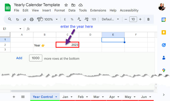
Currently, it contains the year 2023. If you wish to generate the 12-month calendar for the year 2024, simply replace 2023 with 2024 in cell C2.
How to Use the Dynamic Yearly Calendar Template in Google Sheets:
Please refer to the screenshot of the January month’s calendar.
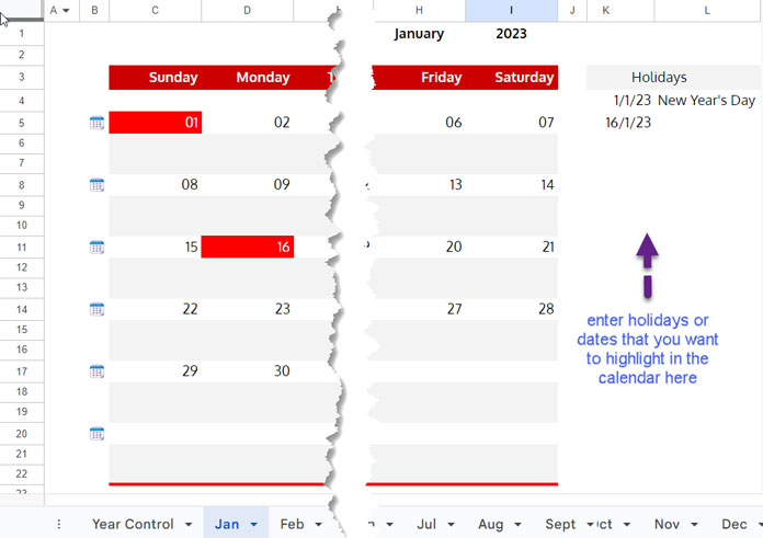
- Highlighting Dates: If you want to emphasize any date in the calendar, such as holidays, upcoming birthdays, or other events like marriages and business meetings, enter them in column K under holidays.
- Personal Notes: There are two blank rows below each week’s dates, highlighted in light grey. You can enter any notes in them. As a side note, you can look up data on another sheet and dynamically display it below each date. Please check my calendar view template for that.
- Column C contains formulas in rows corresponding to the calendar icon in column B.
These usage instructions apply to each month’s calendar in the template.
How to Create a Dynamic Yearly Calendar in Google Sheets
To elucidate the formulas and demonstrate how to create a dynamic yearly calendar template, let’s concentrate on the ‘Feb’ sheet.
If we were to choose the ‘Jan’ sheet, I wouldn’t be able to explain the formula accurately because the first week of January 2023 starts on Sunday.
The calendar template header (C3:I3) contains the days of the week from Sunday to Saturday. Therefore, if we use January, I won’t be able to illustrate how aligning the date in the first week corresponds to the days of the week in the header.
The formula is the same across all sheets, so there’s no need to worry about the sheet we choose for the explanation.
Let’s proceed with the step-by-step instructions to create a dynamic yearly calendar in Google Sheets.
As previously mentioned, cell C2 in the ‘Year Control’ sheet contains the year for the calendar to populate. In cell I1 on the ‘Feb’ sheet, enter the following formula to fetch that year.
='Year Control'!C2In cell H1, input the text “February.” For other sheets, replace this text with the corresponding month names.
In the cell range C3:I3, enter the following days of the week: Sunday, Monday, Tuesday, Wednesday, Thursday, Friday, and Saturday. Please refer to the screenshot below.
Key Formula for Populating Dates in the Calendar Template
In cell C5, enter the following formula:
=SEQUENCE(1, 7, DATE(I1, MONTH(H1&1), 1)-WEEKDAY(DATE(I1, MONTH(H1&1), 1))+1)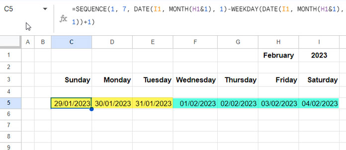
The above formula returns date values (numbers). I’ve formatted them as dates using Format > Number > Date to show you the relevant dates. To format them as days, follow these steps:
- Select the cell range C5:I5.
- Click Format > Number > Custom number format.
- Enter
ddin the given field and click Apply.
This SEQUENCE formula is the key to generating the dynamic yearly calendar in Google Sheets. Let me explain it.
Syntax of the SEQUENCE Function:
SEQUENCE(rows, [columns], [start], [step])Where:
rowsis 1columnsis 7startisDATE(I1, MONTH(H1&1), 1)-WEEKDAY(DATE(I1, MONTH(H1&1), 1))+1
Let’s further break down this start argument.
Section #1:
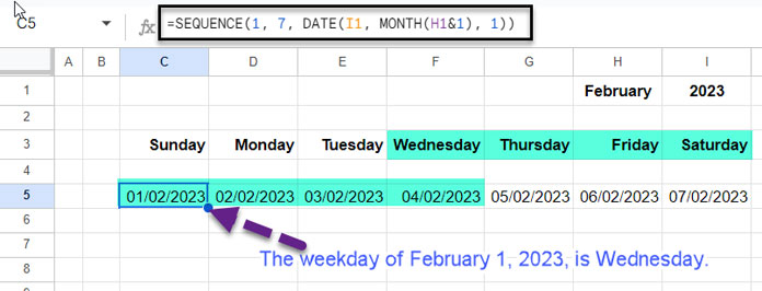
DATE(I1, MONTH(H1&1), 1)This formula calculates the date of the first day of a specified month in a given year. In this case, the result will be February 1, 2023.
Syntax of the DATE Function:
DATE(year, month, day)Where:
year:I1is the cell reference containing the year.month:MONTH(H1&1)converts the month name in cell H1 to a month number.day: 1 is the day number, which is always 1 for the first day of the month.
Section #2:
If we only use section #1 as the start argument, the SEQUENCE formula will return the dates from Wed, 1 Feb 2023 to Tue, 7 Feb 2023. It’s not aligned with the days of the week in the header, which goes from Sunday to Saturday.
How do we align it?
We subtract the weekday number of the start date plus 1 from the start date. Therefore, the start date in the SEQUENCE will become Sunday, January 29, 2023.
DATE(I1, MONTH(H1&1), 1)-WEEKDAY(DATE(I1, MONTH(H1&1), 1))+1We will then hide the unwanted previous month’s dates using a highlighting rule, which we will cover later.
Let’s go to the other formulas used in the dynamic yearly calendar template.
Other Formulas
In cell C8, enter the following formula and then copy-paste it to C11, C14, C17, and C20.
=SEQUENCE(1, 7, I5+1)All of them will return 7 date values starting from the date in the last cell of the previous week. Format them as days, similar to how we have done with the date values in C5:I5.
Note: Similar to the first week, the last week may include dates that fall in another month. We will hide them using conditional formatting rules.
Concealing Dates Across Different Months in the First and Last Weeks
To address this, we need to apply a highlight rule to emphasize certain dates in the first and last weeks of the calendar.
- Select the range C5:I20.
- Click on Format > Conditional formatting.
- Choose ‘Custom formula is’ under the ‘Format rules.’
- Copy and paste this formula into the given field:
=AND(MONTH(C5)<>MONTH($H$1&1), ISDATE(C5)) - Under ‘Formatting style,’ select “white” for text color.
- Click ‘Done.’
The highlight rule is essentially an AND logical test and functions as follows:
MONTH(C5)<>MONTH($H$1&1): Checks whether the month of the date in cell C5 is not the same as the month in cell H1.ISDATE(C5): Verifies whether the value in cell C5 is a date.
If both conditions are evaluated as TRUE, the rule applies the highlighting, changing the text color to white.
C5 is a relative cell reference. Therefore, the rule will apply to all cells in the range to which it is applied, i.e., C5:I20.
The above steps are crucial in our dynamic calendar template and should be followed. The subsequent highlighting is optional.
Highlighting Holidays or Other Specific Days in the Yearly Calendar Template
This is the final step in creating the dynamic yearly calendar in Google Sheets.
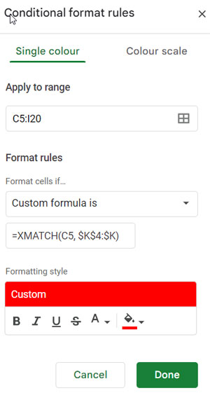
Our dynamic calendar template has a feature that allows you to highlight specific days in the calendar. You need to enter those dates in column K.
To apply that rule, insert the following formula in the custom formula field:
=XMATCH(C5, $K$4:$K)Syntax of the XMATCH Function:
XMATCH(search_key, lookup_range, [match_mode], [search_mode])Where:
C5is thesearch_key$K$4:$Kis thelookup_range.
All the steps are the same as we have done with our previous rule, except for the formula and the fill color. Please refer to the screenshot below.
The XMATCH function matches C5 with the dates listed in column K. Here also, C5 is relative, so it will apply to all cells in the specified range.
Conclusion
I’ve explained how to use our dynamic yearly calendar template in Google Sheets as well as how to create one on your own.
The creation part is intended to assist you in customizing the template according to your requirements. When you insert new rows, delete rows, or change cell colors, understanding the existing formulas will guide you in making the necessary adjustments.
If you have any doubts, please feel free to leave a comment.
Browse our full collection of free Google Sheets templates here.


How can I make the first day of every week to be Monday rather than Sunday?
Change the values in C3:I3 from Sunday to Saturday to Monday to Sunday. Then replace the C5 formula with the following one:
=SEQUENCE(1,7,DATE(I1,MONTH(H1&1),1)-WEEKDAY(DATE(I1,MONTH(H1&1),1), 2)+1)The sheet will adjust the dates automatically.
Thank you! And…if I want the week of the year number to show at the beginning of each week, is that possible? 2024 has 52 weeks plus 1 starting on December 30th.
That requires an additional formula.
Insert the formula below in cell C6. Then copy the formula from that cell and paste it into cells C9, C12, C15, C18, and C21.
Formula:
=ArrayFormula(LET(dt, DATE($I$1,MONTH($H$1&1),1), alldt, SEQUENCE(DAY(EOMONTH(dt, 0)), 1, dt), tbl, SORTN(HSTACK(alldt, WEEKNUM(alldt, 2)), 6, 2, 2, 1), lp, XLOOKUP(C5:I5, CHOOSECOLS(tbl, 1), CHOOSECOLS(tbl, 2),), IF(lp, "Week #"&lp,)))The formula will return the week numbers (Monday-Sunday considered).
I’ve updated this template. Now, you can enter values below dates. The formulas are entirely different. I’ve updated the tutorial accordingly.
I need to make a calendar that runs from July to June on one spreadsheet. I can’t find the section in the formula that requires that the year-end in December every time. Where can I tell it to allow my year to end in June?
Hi, Carrie,
Please check my Fiscal Year calendar template. I have included the link to that post in my reply to another reader earlier. Go through the comments, please.
Best,
Hey! Thanks for the great guide!, I’m having some problems with the final formal #5b, I typed everything correctly as provided, and on the Google Sheet the input is showing as valid, but nothing is appearing in the cells. Any advice on what’s going wrong/what to do?
Also, I was wondering if there is a way to make spaces under each date. I’m using the calendar to make a signup schedule from whose going what days to work in my lab and wanted to leave some cells to let people type in their names. Would I be able to just insert more rows or would I have to adjust the formulas themselves?
Thank you!
-Alexandra Rose
Hi, Alexandra Rose,
I have included the link to my calendar template within this tutorial. I could see that link just below the in-content video player. If you have missed that please have a look at it and make a copy. Then you can check the formula.
“I was wondering if there is a way to make spaces under each date…”
Sorry! It’s not possible.
Best,
Excellent work, but I was wondering if you have a template that shows from one month of one year to the same month of the following year?
Example: From 01st April 2019 – 31st of March 2020
Hi, Martin,
I don’t have such a template. I will definitely consider creating such a calendar template later.
Hi, Martin,
I have created a new calendar. Please do search ‘Fiscal Year’ on this site. See the search button on the top navigation (menu) bar.
Hi!
Thanks for your work! It is very useful.
Is it possible to automatically mark Saturday and Sunday with a different color?
Thanks,
Kukukk
Hi, Kukukk,
You can do that. But there should be 4 rules in the conditional formatting.
That means rule 1 for the range A4:Y9, rule 2 for the range A14:Y19, rule 3 for the range A24:Y29 and rule 4 for the range A34:Y39.
This is the custom formula for rule 1, that means the “Apply to range” in Format > Conditional Formatting” is A4:Y9.
=and(OR(WEEKDAY(A4)=7,WEEKDAY(A4)=1),LEN(A4))This you can use to conditionally format every Sundays and Saturdays with the same color.
If you want a different color, again you may need to split this rule to two as below.
For Saturdays;
=and(WEEKDAY(A4)=7,LEN(A4))For Sundays;
=and(WEEKDAY(A4)=1,LEN(A4))Replace the comma with semicolon as per you Sheets Locale.
Best
It’s working.
Thank you very much!
Hi Prashanth,
Thanks for your work.
I have a problem with your formula #4.
I’m using the Google Sheets french version.
Can you help me?
Thanks in advance for any help.
Best regards
Ossy
Hi, Ossy,
Sorry to hear that you have an issue with the formula. It can be due to the following.
1. The double/single quotes in my formula must be removed and retyped. It’s formatted by my theme’s editor 🙁
2. Your Sheets Locale setting affects the formula. For example, the comma and semicolon must be replaced as detailed below.
Tips: How to Change a Non-Regional Google Sheets Formula.
I know it’s time taking effort for you. So, I have made one copy of my template and changed the locale to France and the formula looks like as below.
=ArrayFormula(if(weekday(D3;1)=1;D3:AH3;{if(weekday(D3;1)=7;{""\""\""\""\""\""};if(weekday(D3;1)=6;{""\""\""\""\""};if(weekday(D3;1)=5;{""\""\""\""};if(weekday(D3;1)=4;{""\""\""};if(weekday(D3;1)=3;{""\""};if(weekday(D3;1)=2;""))))))\D3:AH3}))I have already shared my Calendar template in the post. Open that and make a copy. Then go to the File menu in that sheet and access “Spreadsheet Settings”. There change the Locale to France. You will get the converted formula in cell D5 in the ‘Master Sheet1’ Tab as above.
Hope this helps?
Hi Prashanth
Thanks a lot for your help.
Now everything is working.
You are the best.
Best regards
Ossy
Wow this was amazing! Incredible work and thank you so much!
However, if I want to show the months of July 2019-July 2020 in the Master template, how do I change the formulas? 🙂
Hi Lucas,
I am glad that you liked it.
You can only change the starting month. See the instructions tab point # 4.
Cheers!
Hi, Lucas,
Here you go!
https://infoinspired.com/google-docs/spreadsheet/fully-flexible-fiscal-year-calendar-in-google-sheets/