Get a flexible fiscal year calendar in Google Sheets that you can adjust according to the fiscal year (financial year) in your country.
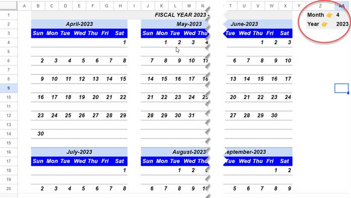
Simply provide the starting month and year of the fiscal year in this calendar template. The well-coded formula in the sheet will then populate a 12-month fiscal year calendar accordingly.
For instance, if you input 4 (April) as the month and 2019 as the year, the calendar will reflect the fiscal year starting from 01-Apr-2019 to 31-Mar-2020. Similarly, entering 1 (January) as the month and 2020 as the year will generate the calendar year 2020 spanning from 01-Jan-2020 to 31-Dec-2020.
It’s important to note that the start date of the fiscal year varies by country worldwide. In the United States, for example, different fiscal years (start months) are followed for various purposes:
| Purpose | Starting Month of the Fiscal Year | Ending Month of the Fiscal Year |
| Federal | October | September |
| Most states | July | June |
| Corporate/personal | January | December |
Fiscal years also differ in the UK, India, Japan, Australia, Germany, France, etc. The flexibility of my Google Sheets fiscal year calendar template allows you to adapt it to the fiscal year conventions of any country.
As it populates a fiscal year calendar based on the starting month, you can use any month to obtain a 12-month calendar accordingly.
My Fiscal Year Calendar Features and Copy
Most of the features have already been mentioned, but let’s summarize them for clarity:
- Free to Use: The Fiscal Year Calendar is free to use in Google Sheets.
- Adaptable: The calendar adapts to the financial year of your specific country.
- Calendar Year Template: It can also be used as a standard calendar year template.
- Flexible Dates: Simply enter the fiscal year start month and year to generate a 12-month calendar across two years.
- Efficient Code: The formula cleverly populates a full month’s calendar, but we’ve designed it to return each week separately. This allows users to enter notes under each week conveniently.
Get The Financial Year Calendar for Any Country:
Here you can preview and copy my financial year calendar. The instructions to use the calendar follows:
How to Use the Financial Year Calendar in Google Sheets
I hope you’ve already copied the sheet. Simply open it and navigate to the “Fiscal Year” tab. In cell AA1, enter the fiscal year start month, and in cell AA2, enter the year. That’s all you need to do.
I’ve left a blank row below each week in every month for you to add notes related to those dates. Feel free to insert additional rows if needed, the formula will automatically adjust.
What about the formula used to create the fully flexible fiscal year calendar in Google Sheets? Let’s explore that under the sub-title below.
Formula to Populate a Calendar for Any Month in Proper Rows and Columns
In the above-shared fiscal year calendar template, you can find a tab named “Drop-Down.” In that sheet, there is a monthly calendar that adjusts based on the month in cell A2 and the year in cell B2.
Here is the dynamic calendar formula in cell C3:
=LET(
   start, C$1,
   seq, SEQUENCE(DAY(EOMONTH(start, 0))),
   test,
      IF(WEEKDAY(start)=1, seq,
      VSTACK(WRAPCOLS(,WEEKDAY(start)-1), seq)
   ), IFERROR(WRAPROWS(test, 7))
)
I used the same formula to create the fiscal year calendar, with one modification. In the fiscal year calendar template, we want blank rows below each week for entering notes.
Since the formula populates a full month’s calendar with proper rows and columns offset, note entering is not possible as is. Therefore, in the fiscal year calendar template, the last part of the formula IFERROR(WRAPROWS(test, 7)) is replaced with IFERROR(CHOOSEROWS(WRAPROWS(test, 7), 1)) in B4, IFERROR(CHOOSEROWS(WRAPROWS(test, 7), 2)) in B6, and so on. The other change is replacing C$1 with B$2.
For a detailed breakdown of the formula, please refer to “Create Monthly Calendars in Google Sheets (Single & Multi-Cell Formulas).”
Related:


This is great but now how can I add info under each date?
The calendar can’t be used to mark anything as each cell only contains the date from formula.
I want to use a FY calendar to mark payment dates (invoices paid to me) and see a yearly overview of when these were paid.
This calendar is useful to set the year and month, but cannot be used for anything other than reference of dates.
Hi James,
Apart from setting the year and month, you can highlight custom holidays by entering them under the range Z5:Z within the sheet ‘Fiscal Year’.
This range can also be utilized to mark payment dates. For a yearly overview, you can, of course, then use the dates under Z5:Z.
If you wish to have both holidays and payments highlighted using different colors, follow the instructions below:
1. Use the existing range Z5:Z for marking/highlighting official holidays (red color).
2. Use the range AE5:AE for marking/highlighting payment dates (green color).
I have already made the changes to the sheet.
Unfortunately, there is no option to directly insert notes within the calendar, as I have employed a single formula to populate an entire month’s calendar with proper weekday offsetting.
I hope this clarifies.
I’ve updated the template; now there are blank rows below each week.