In this post, we will provide an hourly time slot booking template in Google Sheets along with the formulas used to create it.

Here’s how it works: you select a start date to view the status of booked time slots in that week for various items. The items can include car/bike/equipment rental, tasks, hourly-based room booking, or anything that you allow booking on an hourly basis.

The template operates as follows: choose the item from column A, enter the start datetime and end datetime in columns C and D. Then, select whether the booking is confirmed or tentative in column F.

In another sheet, you can view the booked status in a bar chart with two distinguishable colors: orange represents tentative bookings, and green represents confirmed bookings.

Below, I’ll provide you with a free download link to my hourly time slot booking template in Google Sheets and instructions on how to use it.

Additionally, you will receive all the formulas and explanations. These will enable you to modify the template, such as inserting or moving columns in the input sheet.

Explore Our Intuitive Dynamic Hourly Time Slot Booking Template Interface

Our hourly time slot booking template in Google Sheets consists of two sheets: “Bookings” and “Status.” You can preview and copy it using the following template preview link.

Template

Let’s begin by exploring the “Status” sheet.

Status Sheet

Begin by entering all the items available for booking in the range A4:A. You can replace the existing items and add new ones as needed. Please ensure there are no duplicates.

Highlighting occurs within the “Status” sheet as follows:

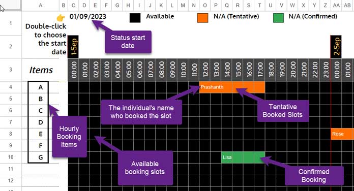
• Available Time Slots: Black-colored cells in the grid represent available booking slots.
• Booked Slots: Orange-highlighted cells represent tentative bookings, and green-highlighted cells represent confirmed bookings.

Since this is an hourly time slot booking template, each cell in the grid represents one hour.

The name of the individual who booked the time slot will appear in the very first cell. If a person booked for 2 hours, the highlighting will span two cells, and the first cell will contain their name.

There is a specific reason for displaying individuals’ names in our hourly time slot booking template. Without names, it would be challenging to identify the start time of the second person’s booking if, for instance, one person booked from 10:00 to 12:00 and another from 12:00 to 18:00.

You can select the status start date by double-clicking on cell C1. The bars in the grid and the date/time in the chart timescale at the top will refresh accordingly. The template is set to display 7 days from the selected date, resulting in 168 (7 x 24) time slots in each row for each item.

In summary, input all the available booking items in cells A4:A and select a start date from cell C1. The formulas will handle the rest.

Booking Sheet

This is the second sheet in our hourly time slot booking template in Google Sheets.

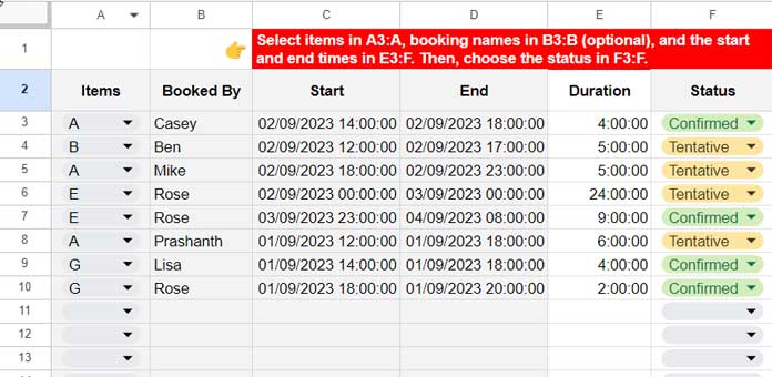
The drop-down lists in cell range A3:A will display the items you entered in range A4:A on the “Status” sheet. Therefore, please ensure that you enter all the items available for booking in the “Status” sheet’s range A4:A.

Select an item in cell A3. Enter the booked person’s name in cell B3, followed by the booking start time (timestamp) and end time (timestamp) in C3:D3.

Remember, ours is an hourly time slot booking template, so you should only enter the hour component in the time, skipping seconds and minutes.

Then, select either “Tentative” or “Confirmed” in cell F3.

Continue this process in the rows below.

That’s all you need to input in the “Booking” sheet of our hourly time slot booking template in Google Sheets.

Observing the following points when inputting data in the “Booking” sheet will help you generate correct status bars in the “Status” Sheet.

• Start and End times must be timestamps.
• Minutes and seconds are not supported in the start and end times.
  • If a person booked for 1 hour, it should be like this:
    • Start: 02/09/2023 14:00:00
    • End: 02/09/2023 15:00:00
  • Not like this:
    • Start: 02/09/2023 14:00:00
    • End: 02/09/2023 14:00:00.
• Before booking, refer to the “Status” sheet for available time slots to avoid errors, such as overlapping dates in the same item booking.

Formulas Utilized in the Hourly Time Slot Booking Template in Google Sheets

I haven’t used any scripts in our template. I’ve utilized native functions within the sheet for highlighting and other purposes. All the formulas are array formulas, meaning they will automatically adjust as your data grows. You don’t need to worry about dragging down the fill handle or copying and pasting them.

Here are the formulas used in our hourly time slot booking template in Google Sheets.

Highlight Rules

There are two conditional format rules in the “Status” Sheet for plotting the bars.

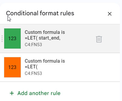
1. Confirmed Booking of Time Slots (Green)

The following formula is used within Format > Conditional format > Custom formula rule for the “Apply to range” C4:FN53 to plot the green color bars that represent confirmed time slot bookings.

=LET(
     start_end, "Booking!C3:D", 
     booked_item, "Booking!A3:A", 
     status, "Booking!F3:F", 
     item, $A4, 
     datetime, C$3, 
     ftr, 
     FILTER(INDIRECT(start_end), (INDIRECT(booked_item)=item)*
     (INDIRECT(status)="Confirmed")), 
     SUM(
        MAP(CHOOSECOLS(ftr, 1), INDEX(CHOOSECOLS(ftr, 2)-TIME(1, 0, 0), 0), 
        LAMBDA(st, en, N(ISBETWEEN(datetime, st, en))))
     )
)

Formula Breakdown:

We used the LET function to define names for ranges, making the formula more readable and efficient. Here are the defined names and value expressions:

• start_end: “Booking!C3:D”
• booked_item: “Booking!A3:A”
• status: “Booking!F3:F”
• item: $A4
• datetime: C$3
• ftr: FILTER(INDIRECT(start_end), (INDIRECT(booked_item)=item)*(INDIRECT(status)="Confirmed"))

The formula expression is as follows:

SUM(MAP(CHOOSECOLS(ftr, 1), INDEX(CHOOSECOLS(ftr, 2)-TIME(1, 0, 0), 0), LAMBDA(st, en, N(ISBETWEEN(time, st, en)))))

The MAP function tests whether the time in the “Status” sheet C3 is between the filtered start and end datetimes (ftr) in each row, returning an array of zeros and ones. The SUM function totals the result. If it’s >0, the corresponding time slot below C3 is highlighted.

In the formula, cell references $A4 and C$3 use a combination of relative and absolute cell references.

This configuration ensures that each cell in the grid is tested and highlighted appropriately as the formula is extended to different cells within the sheet.

2. Tentative Booking of Time Slots (Orange)

This is essentially a copy of the above formula. The only difference lies in the criteria part of the FILTER function, where we replaced INDIRECT(status)="Confirmed") with INDIRECT(status)="Tentative").

Formula to Display Names in the Status Bar

One distinctive feature of our hourly time slot booking template is the presentation of the names of booked individuals on the time slots within the bar. This feature facilitates distinguishing between continuous bookings of time slots by different individuals.

To achieve this, the following formula is employed in cell C4 on the “Status” sheet:

=LET(
   datetime, C3:3, 
   item, A4:A, 
   name, Booking!$B$3:$B, 
   r_item, Booking!$A$3:$A,
 
   start, Booking!$C$3:$C, 
   MAP(datetime, LAMBDA(c, MAP(item, LAMBDA(r, 
      JOIN(" ?", IFNA(FILTER(name, (r_item=r)*(start=c))))
   ))))
)

Formula Breakdown:

Defined names and value expressions in the LET function:

• datetime: C3:3
• item: A4:A
• name: Booking!$B$3:$B
• r_item: Booking!$A$3:$A
• start: Booking!$C$3:$C

The formula expression is as follows:

MAP(datetime, LAMBDA(c, MAP(item, LAMBDA(r, JOIN(" ?", IFNA(FILTER(name, (r_item=r)*(start=c))))))))

The formula is straightforward to understand. The FILTER function filters the names of individuals who booked time at a particular time (C3) and for a specific item (A4).

To cover each row (C3:3) and column (A4:A), two MAP functions are utilized.

Dynamic Timescale for the Hourly Time Slot Booking Template

In cell C3 of the “Status” sheet, the following formula generates datetimes for the hourly time slot booking template:

=ARRAYFORMULA(C1+SEQUENCE(1, 7*24, 0)/24)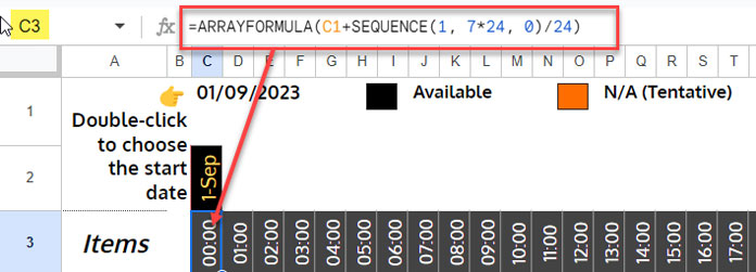

I’ve formatted the range C3:3 to “HH:MM” using Format > Number > Custom date and time.

The SEQUENCE function produces numbers from 1 to 168. By dividing these numbers by 24 and adding the result to the date in cell C1, we obtain the desired datetime values.

Optional Formulas in the Hourly Time Slot Booking Template

There are two optional formulas: one in Status!C2 and the other in Booking!E2.

Formula in C2 (Status Sheet):

The formula shows the dates for each 24 hours in the timescale.

=ArrayFormula(IF(MOD(C3:FN3, 1)=TIME(0, 0, 0), INT(C3:FN3),))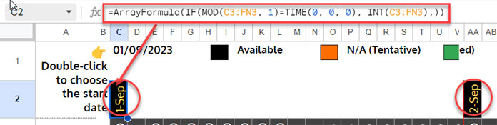

Explanation:

• The MOD function, MOD(C3:FN3, 1), extracts the time component from the datetime values in cells C3 to FN3. The IF function evaluates the extracted time values and returns the corresponding dates in cells C3 to FN3 wherever the MOD function returns 00:00.

Formula in E2 (Booking Sheet):

This formula returns the duration from the time slot booking start and end datetimes:

=ARRAYFORMULA(VSTACK("Duration", IF(A3:A="",,D3:D-C3:C)))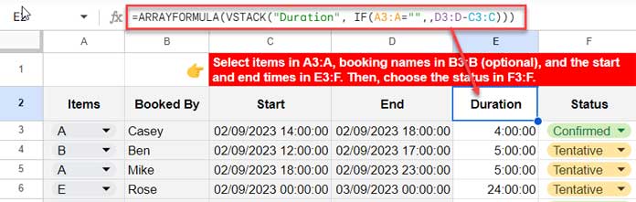

Explanation:

• IF(A3:A="",,D3:D-C3:C): Calculates the duration only if there is a booking (if A3:A is not empty).
• VSTACK("Duration", …): VSTACK stacks the label “Duration” above the calculated durations.

Conclusion

In conclusion, this user-friendly and efficient hourly time slot booking template in Google Sheets simplifies the process of managing appointments and reservations.

This version is an extension of our Reservation and Booking Status Calendar Template in Google Sheets, designed for per-day booking management.

Both templates feature an intuitive design and automated features, making scheduling a breeze.

Feel free to customize and utilize this hourly time slot booking template to streamline your time management, ensuring a seamless and organized booking experience for both you and your clients.

Enhance productivity and eliminate scheduling hassles with this convenient tool at your fingertips.