You can create monthly calendars in Google Sheets using either a single formula for the entire month or multiple formulas for each week.

The former is best if you want to print or refer to calendars within the Sheet, and the latter is useful when you want blank rows between each week for entering notes.

When creating a monthly calendar using a single formula, one of the hurdles you may face is skipping or offsetting the first date in a month to the correct day of the week column.

I offer a unique solution for creating a dynamic monthly calendar in Google Sheets using single and multi-cell formulas.

How to Create a Monthly Calendar Using a Single Formula in Google Sheets

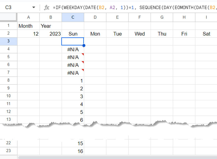
Enter the month number in cell A2 and the year in cell B2.

Then, input the days of the week from Sunday to Saturday in cells C2:I2.

To create the monthly calendar, enter the following array formula in cell C3:

=LET(
   start, DATE(B2, A2, 1), 
   seq, SEQUENCE(DAY(EOMONTH(start, 0))), 
   test, 
      IF(WEEKDAY(start)=1, seq, 
      VSTACK(WRAPCOLS(,WEEKDAY(start)-1), seq)
   ), IFNA(WRAPROWS(test, 7))
)

This formula will generate the entire month’s calendar at once!

It’s a magical formula; you don’t need to format the result, apply conditional formatting to mask dates, or anything else. The formula will take care of everything.

When you enter a new month number in cell A2, the calendar will refresh. The same is true for the year in cell B2. You can also use data validation drop-downs in cells A2 and B2 to quickly select the month and year.

Monthly Calendar Formula Breakdown (Unleash the Power of Dynamic Calendars)

Some of you may want to learn the formula to improve your Google Sheets skills. Here is how the single formula dynamically populates a full month’s calendar in one go with the proper weekday offset in the first row.

There are four major parts in the formula that create a dynamic monthly calendar in Google Sheets: Sequence Part, Offset Part, Combining Offset and Sequence, and Wrap to Rows Part.

Sequence Part: Creating a Sequence of Days in the Month

First of all, we need to find the month start date from the month and year in cells A2 and B2. The following formula does that:

=DATE(B2, A2, 1)

Now, we need to determine the total days in that month. For that, we find the month-end date using the EOMONTH function:

=EOMONTH(DATE(B2, A2, 1), 0)

If we wrap the above formula with the DAY function, we get the last day in the selected month and year:

=DAY(EOMONTH(DATE(B2, A2, 1), 0))

Wrap it with SEQUENCE to get the days in the whole month, i.e., sequence numbers from 1 to the total days in the month:

=SEQUENCE(DAY(EOMONTH(DATE(B2, A2, 1), 0)))

Offset Part: Adjusting Days Based on the Days of the Week

This is a key part of creating a dynamic monthly calendar using a single formula in Google Sheets.

If the month start date begins on Sunday, we need to offset the above sequence by 0 cells. If it starts on Monday, offset by 1 cell, and so forth. How do we do that?

=WEEKDAY(DATE(B2, A2, 1))-1

The above WEEKDAY formula will return the number to offset. It returns the weekday number – 1, resulting in 0 for Sunday, 1 for Monday, and so on.

Wrapping it with the WRAPCOLS function, as shown below, will return n error cells, and that is the Offset Part:

=WRAPCOLS(,WEEKDAY(DATE(B2, A2, 1))-1)

Combining Offset (N Error Cells) and Sequence (Days in a Month)

Next, we want to stack it (Offset Part result) with the sequence numbers (Sequence Part result) only if the weekday number is not equal to 1 (not equal to Sunday).

Here is the generic formula that uses an IF logical test:

=IF(WEEKDAY(DATE(B2, A2, 1))=1, sequence_part, VSTACK(offset_part, sequence_part))

So the corresponding formula will be:

=IF(WEEKDAY(DATE(B2, A2, 1))=1, SEQUENCE(DAY(EOMONTH(DATE(B2, A2, 1), 0))), VSTACK(WRAPCOLS(,WEEKDAY(DATE(B2, A2, 1))-1), SEQUENCE(DAY(EOMONTH(DATE(B2, A2, 1), 0)))))

Wrap to Rows Part: The Final Step in Creating a Dynamic Monthly Calendar in Google Sheets

To create the dynamic monthly calendar, you just need to use the WRAPROWS function to wrap the above formula to wrap the output by 7 cells and use IFNA to replace error cells with blank.

=IFNA(WRAPROWS(IF(WEEKDAY(DATE(B2, A2, 1))=1, SEQUENCE(DAY(EOMONTH(DATE(B2, A2, 1), 0))), VSTACK(WRAPCOLS(,WEEKDAY(DATE(B2, A2, 1))-1), SEQUENCE(DAY(EOMONTH(DATE(B2, A2, 1), 0))))), 7))

That is our single-cell formula for creating a dynamic monthly calendar in Google Sheets.

But you will notice a different formula before the sub-title ‘Monthly Calendar Formula Breakdown’ above. That’s because we have used the LET function there, so that we can avoid using the same expressions more than once in the formula, for example, the SEQUENCE and DATE.

Creating a Monthly Calendar Using Separate Formulas for Each Week

If you want blank rows between each week in the calendar, you need to resort to separate formulas for each week.

Don’t worry; we have a single-cell magical formula that creates a dynamic monthly calendar in Google Sheets. You need to use the CHOOSEROWS function with it to choose the row you want.

In our one-piece code for the whole month, we need to replace the IFNA(WRAPROWS(test, 7)) part with IFERROR(CHOOSEROWS(WRAPROWS(test, 7), n)).

The n will be 1 in the first row, 2 in the second row, and so forth. You need n up to 6.

=LET(
   start, DATE(B2, A2, 1), 
   seq, SEQUENCE(DAY(EOMONTH(start, 0))), 
   test, 
      IF(WEEKDAY(start)=1, seq, 
      VSTACK(WRAPCOLS(,WEEKDAY(start)-1), seq)
   ), IFERROR(CHOOSEROWS(WRAPROWS(test, 7), n))
)

Conclusion

You might have come across various formulas in Excel as well as Google Sheets for creating a monthly calendar or template. Our formula stands out from the rest due to its simplicity and flexibility.

Many of the formulas offered use multiple formulas, which may require additional steps like highlighting or formatting.

In our case, you can use the formula straight out of the box. Simply insert the month and year into designated cells (A2 and B2), type the days of the week from Sunday to Saturday in C2:I2, and copy-paste our formula. The formula will take care of the rest.

You can also split the same formula into multiple rows using the CHOOSEROWS function. If you are interested in customized templates, check out these tutorials:

• Calendar View in Google Sheets (Custom Template)
• Hyperlink Calendar Dates to Events in Google Sheets
• Reservation and Booking Status Calendar Template in Google Sheets
• Hourly Time Slot Booking Template in Google Sheets