A calendar view template in Google Sheets can help you view your data (records) in an easy-to-understand way.
In Google Sheets, we can create and view reports in tabular form using functions like FILTER, QUERY, or Pivot Table.
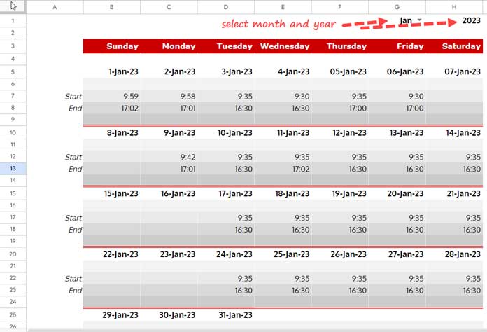
However, the custom calendar view mode in Google Sheets displays the information in a standard calendar format—based on the user-selected month and year, and other settings within the source data sheet.
You can navigate through the calendar by month and year.
The corresponding data will be displayed under each date in the selected month and year, depending on the availability of data in the source sheet.
You can use my template to view sales data, purchase data, employee punch data, to-do lists, track your events and meetings, and more.
Features
The custom calendar view template supports different data types. They are text, numbers, time, and duration.
If multiple records are present for a date, the data will be aggregated based on the data type.
- Numbers and durations will be summed.
- Texts will be made unique and then concatenated.
Combining multiple columns is also supported.
It’s useful when you have things like name, email, and phone number entered in separate columns.
We’ll see more about these features in the example section below. Before that, you can download (make a copy of) my calendar view template:
Using a Custom Calendar View Template in Google Sheets
The template file has two sheets: Master and CV.
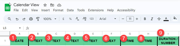
The Master sheet contains nine preset fields (columns):
- Column 1: Date
- Columns 2 to 6: Text
- Columns 7 and 8: Time
- Column 9: Duration or number
Note: If you’re entering durations (like overtime), make sure the column is formatted as Format > Number > Duration. A time difference likeEnd Time - Start Timemay show correctly but won’t be treated as a duration unless the format is set.
Required Fields in Master Tab
You only need to fill in the necessary columns. The CV sheet will automatically update to reflect the data in the Master sheet.
Note: The values entered in columns 2 to 6 will be combined into a single value in the calendar.
Let’s see three examples.
Example 1: Employee Time Tracking
As we saw above, the Master sheet is formatted to support different data types. We’ll start by entering the punching data of an employee.
To create a daily time calendar, we need three fields: Date, Start Time, and End Time.
We’ll enter data in columns A, G, and H (columns 1, 7, and 8 respectively).
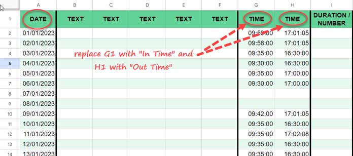
Remove the field labels in the unused columns B1:F1 and I1.
Notes:
- If an employee has multiple in/out records for the same date, the earliest time will be treated as time in, and the latest as time out.
- You’ll need to manually enter the texts
"Start"and"End"in column A of the CV sheet, in the respective rows. (Refer to the image below.)
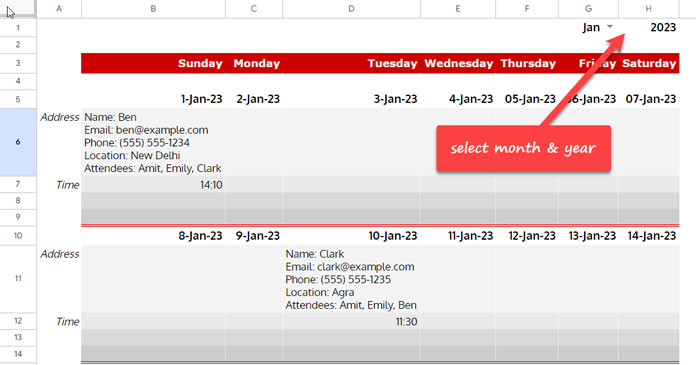
Example 2: Appointment Log
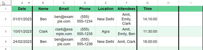
In this example, we want to display an appointment log. So, the input will include these fields:
- Date (Column 1)
- Name (Column 2)
- Email (Column 3)
- Phone (Column 4)
- Meeting Location (Column 5)
- Attendees (Column 6)
- Time (Column 7)
Fill in the relevant fields in the Master sheet.
Once the data is ready, go to the CV sheet to view the calendar.
Example 3: To-Do List View
Having a to-do list is a good way to stay on top of personal or work-related tasks.
If you already use a spreadsheet—or are planning to—Google Sheets is a great option.
Do you know why?
Because it’s cloud-based. You can access it from your mobile or desktop, whether you’re at home or at work.
You can use my template to enter your to-do list and view them in calendar form.
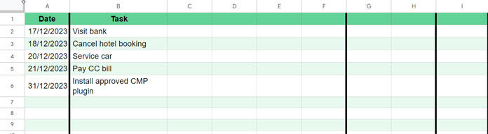
In the Master sheet:
- Enter task dates in Column A
- Enter task names in Column B
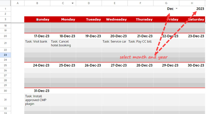
Then go to the CV sheet and select the month in cell G1 and the year in cell H1.
That’s it—your to-do list will appear under the corresponding dates.
Key Formulas in the Template
We have several array formulas in the CV sheet, mostly in the range B5:B34.
- B5, B10, B15, B20, B25, and B30: These build the calendar structure dynamically.
- The cells right below each (like B6 to B9) retrieve the actual data to display.
Let’s go through the important ones.
B6: Text Values from Columns B to F (2 to 6)
This formula pulls in and combines text from multiple columns:
=ARRAYFORMULA(
  LET(
    source_dt,   Master!$A$2:$A,
    source_txt,  Master!$B$2:$F,
    header,      Master!$B$1:$F$1,
    month_txt,   $G$1,
    calendar_dt, B5:H5,
    MAP(calendar_dt, LAMBDA(dtd,
      TEXTJOIN(CHAR(10), TRUE,
        UNIQUE(IFNA(
          FILTER(
            IF(LEN(source_txt), header & ": " & source_txt, ),
            DATEVALUE(source_dt) = dtd,
            MONTH(source_dt) = MONTH(month_txt & 1)
          )
        ))
      )
    ))
  )
)
It uniques and combines the texts.
B7: Earliest Time from Column G (7)
=ARRAYFORMULA(
  LET(
    source_dt, Master!$A$2:$A,
    numeric,   Master!$G$2:$G,
    month_txt, $G$1,
    calendar_dt, B5:H5,
    MAP(calendar_dt, LAMBDA(dtd,
      SORTN(IFNA(FILTER(numeric, DATEVALUE(source_dt)=dtd, MONTH(source_dt)=MONTH(month_txt&1))))
    ))
  )
)
It returns the earliest time for a given date.
B8: Latest Time from Column H (8)
=ARRAYFORMULA(
  LET(
    source_dt, Master!$A$2:$A,
    numeric,   Master!$H$2:$H,
    month_txt, $G$1,
    calendar_dt, B5:H5,
    MAP(calendar_dt, LAMBDA(dtd,
      SORTN(IFNA(FILTER(numeric, DATEVALUE(source_dt)=dtd, MONTH(source_dt)=MONTH(month_txt&1))), 1, 0, 1, 0)
    ))
  )
)
It returns the latest time when there are multiple records for the same date.
B9: Duration or Number from Column I (9)
=ARRAYFORMULA(
  LET(
    source_dt, Master!$A$2:$A,
    numeric,   Master!$I$2:$I,
    month_txt, $G$1,
    calendar_dt, B5:H5,
    result, MAP(calendar_dt, LAMBDA(dtd,
      IFNA(SUM(FILTER(numeric, DATEVALUE(source_dt)=dtd, MONTH(source_dt)=MONTH(month_txt&1))))
    )),
    IF(result > 0, result, )
  )
)
It sums the values when there are multiple entries for the same date.
I’ve copied the formulas in B6 to B9 together and pasted them into B11, B16, B21, B26, and B31 (the first row of each group) to cover the rest of the calendar rows.
Tips for Customization
I’ve given three examples to show how to use this template.
In all of them, we didn’t use the 9th column (duration/numeric) from the Master sheet. Here’s how to use it.
Let’s say you want to track your daily expenses.
In the Master sheet:
- Enter the date in Column A
- Enter the expense head (description) in Column B
- Enter the amount in Column I
If you have more than one expense on the same day, you can:
- Add them in two rows, and the formula will aggregate (sum) them.
- Or combine the descriptions in one row (comma-separated), manually total the amount, and enter it in Column I.
You can use this same logic for tracking durations—like daily overtime.
Once you go through the three examples above, adding this will feel natural.
That’s all about the calendar view template in Google Sheets. I hope you found it useful.
More Google Sheets Templates You Might Like
- Calendar Heatmap in Google Sheets (Free Template + How to Use)
- Content Calendar Template in Google Sheets (Free, Dynamic & Fully Automated)
View all our Google Sheets templates in one place.


Could you please explain how to get data to enter into the next colored row for each day? Right now, all my entries for a day stay in the first row and grow downward instead of filling the cells below. How do I move data into the second row for a specific day?
Each row in this calendar view is designed for a specific purpose: the first row is for text, the second and third rows are for “Time In” and “Time Out,” and the fourth row is for numbers or duration.
Please ensure your data is organized to match this structure so it populates the rows correctly.
If I’m not using rows 2–4, can they be removed from the calendar view?
Also, if there is more than one event on a single day, is there a way to display additional events in subsequent rows?
You can remove those rows if you’re not using them.
As for displaying multiple events on the same day in separate rows, that isn’t very practical. There’s no way to predict how many rows would be needed under a single date. From a design perspective, combining the events into a single cell is the most reliable approach—and that’s the method I’ve followed here.
Prashanth,
I came across your brilliant Google Sheet via this discussion thread:
https://support.google.com/docs/thread/250378544/autofill-data-and-date-range-entered-in-google-sheets-into-another-sheet-containing-calendar?hl=en
I want to use the Calendar View to draw data from many tabs containing marketing tasks across various dates. Is there a way to automatically fill the Master sheet with data from multiple tabs?
Also, the information I’m trying to pull includes these columns: Start Date, Due Date, Task, Campaign, Type (eBlast vs. Social Media). One more note—each tab currently has a long name. I’d be happy to share this Google Sheet with you as well.
Jeanne
Thanks, Jeanne!
You can follow this tutorial — Combine Data Dynamically in Multiple Tabs Vertically in Google Sheets — to stack data from multiple tabs into the Master sheet automatically. It walks through how to consolidate data from tabs with similar structures.
Hope that helps you get started!