In this walkthrough, let me explain how to hyperlink the results of the FILTER function in Google Sheets.

We typically use the FILTER function to extract specific data from a large dataset. Unlike the FILTER menu, which presents the data directly, using the FILTER function allows us to place the results in a separate range for additional processing.

One drawback of filtering data with the FILTER function is the inability to edit the results directly. Editing requires going back to the source data, and this can be challenging when we don’t know the exact cell from which the data is extracted by the formula.

This is where the relevance of hyperlinking the FILTER function results comes into play. Hyperlinking enables us to click on values in the filter formula results, allowing us to jump directly to the corresponding cell in the filtered result.

This tutorial explains how to use the HYPERLINK function with the FILTER function, and the formula is designed to work seamlessly even with 2D results.

Let’s delve into the formula, and its usage, and then proceed to a detailed explanation of how it works.

Linking Filter Formula Results with Source Data: Sample Data

In the following example, I have source data in the cell range B2:E, which represents the supply status of aggregate materials.

The data is formatted with columns for Item, Qty, Location, and Date. My goal is to filter the records in the table that match the item “Sand” in the first column.

The top row of the table, B2:E2, contains the field labels. Therefore, the filter range is B3:E, and the criteria range is B3:B.

I have entered the criterion “sand” in cell G2.

To filter the records matching the item “Sand,” we can use the following formula in cell H2:

=FILTER(B3:E, B3:B=G2)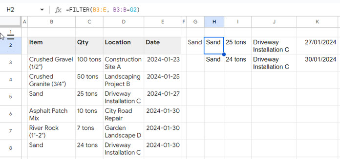

However, the results are not linked to the source data. Although changes in the source data will reflect in the result, we can’t click on the result and jump to the source data.

How can we use the HYPERLINK function with the FILTER function to address this issue?

Using HYPERLINK with FILTER Function: Formula

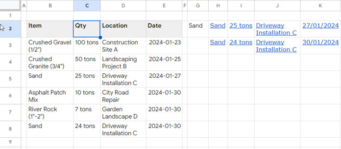
Here is the corrected formula to hyperlink filter results with source data in Google Sheets:

=ArrayFormula(LET(
     f_range, B3:E, 
     c_rangeA, B3:B, 
     cA, G2, 
     ft_row, B3:E3, 
     url, "original_URL_here", 
     HYPERLINK(
          url&
          REGEXREPLACE(ADDRESS(ROW(ft_row), COLUMN(ft_row), 4), "[0-9]", "")&
          FILTER(ROW(c_rangeA), c_rangeA=cA), 
          FILTER(f_range, c_rangeA=cA)
     )
))

In the formula:

• f_range represents the filter range, which is B3:E.
• c_rangeA represents criteria range1, which is B3:B.
• ft_row represents the first row in the f_range, which is B3:E3.
• cA represents criterion1, which is G2.
• url represents the URL of cell A1 in the source data sheet, and you should replace “original_URL_here” with the actual URL.

To obtain the URL, right-click on cell A1 in the source data sheet, select “View more cell actions,” and then click on “Get links to this cell” in the context menu.

Replace the string “original_URL_here” with the just-copied URL and remove A1 from the last part of it. See the example below.

https://docs.google.com/spreadsheets/d/12pYMR3StdSQ6aKyww4x_bgicYKjm59Bv_n_qkyFekTQ/edit#gid=3223244&range=A1 // actual
https://docs.google.com/spreadsheets/d/12pYMR3StdSQ6aKyww4x_bgicYKjm59Bv_n_qkyFekTQ/edit#gid=3223244&range= // requried

If you want to see the HYPERLINK and FILTER combination in action, click on the button below to access the link and copy the sheet.

Sample Sheet

Examples of Filtering Specific Columns and Hyperlinking

The above formula is dynamic. In the example, it filters the records matching the item “Sand.”

How do I filter only the “Location” and “Date” from the table instead, focusing on two specific columns?

You need to make two changes in the formula:

1. Replace B3:E, which is the filter range (f_range), with D3:E.
2. Replace B3:E3, the first row in the f_range, with D3:E3.

What about two distant columns?

Using HYPERLINK with the FILTER function, we can filter distant columns as well. For example, to filter the columns “Item” and “Date” and hyperlink, follow the below approach:

CHOOSECOLS(hyperlink_filter_formula, {column1, column2, ...})

I mean to filter the total records, as per our initial example using the HYPERLINK and FILTER combination, and wrap it with the CHOOSECOLS function to select the required columns in the result.

Filtering and Hyperlinking with Multiple Criteria

When using the HYPERLINK function with the FILTER function, you can include multiple criteria, similar to a regular filter formula.

In the above code, the filter formulas are as follows (yes, we have used two filter formulas):

FILTER(ROW(c_rangeA), c_rangeA=cA)
FILTER(f_range, c_rangeA=cA)

where the criteria range and criterion are:

• c_rangeA is criteria range 1
• cA is criterion 1

You can specify additional criteria ranges and criteria, for example:

FILTER(ROW(c_rangeA), c_rangeA=cA, c_rangeB=cB)
FILTER(f_range, c_rangeA=cA, c_rangeB=cB)

In addition to the above changes, you should specify them within LET as follows at the beginning of the formula. This is the current part:

LET(
     f_range, D3:E, 
     c_rangeA, B3:B, 
     cA, G2, 
     ft_row, D3:E3, 
     url, "url_here",...

After specifying new criteria range and criterion (example):

LET(
     f_range, D3:E, 
     c_rangeA, B3:B, 
     cA, G2, 
     c_rangeB, C3:C, 
     cB, G3, 
     ft_row, D3:E3, 
     url, "url_here",...

That’s all about how to modify the formula to return the full or part of the table and also adding additional conditions. Let’s move on to the formula explanation now.

Formula Breakdown

We have used the LET function to define names for ranges (value expressions).

LET( f_range, D3:E, c_rangeA, B3:B, cA, G2, ft_row, D3:E3, url, "url_here",...

Syntax:

LET(name1, value_expression1, [name2, …], [value_expression2, …], formula_expression)

Let’s proceed to the formula expression part where we hyperlink FILTER function results.

The formula is essentially a HYPERLINK function that uses specific cell addresses to hyperlink with corresponding link labels.

The specific cell address is the address of the filtered values, and link labels are the corresponding values.

Hyperlink Formula:

HYPERLINK( url& REGEXREPLACE(ADDRESS(ROW(ft_row), COLUMN(ft_row), 4), "[0-9]", "")& FILTER(ROW(c_rangeA), c_rangeA=cA), FILTER(f_range, c_rangeA=cA) )

It follows the syntax of HYPERLINK(URL, [link_label]).

Where URL is:

url& REGEXREPLACE(ADDRESS(ROW(ft_row), COLUMN(ft_row), 4), "[0-9]", "")& FILTER(ROW(c_rangeA), c_rangeA=cA)

In this, “url” is the one copied from cell A1, with the removal of the “A1” string from the last part.

REGEXREPLACE(ADDRESS(ROW(ft_row), COLUMN(ft_row), 4), "[0-9]", "") returns the column letters of the range to filter.

FILTER(ROW(c_rangeA), c_rangeA=cA) the first FILTER formula, which returns the row numbers of the filtered rows.

Note: To learn the functions individually, please refer to my Google Sheets function guide.

We combined all these elements (URL, column letters, and row numbers) in an array formula using the ampersand (&) to obtain the URLs of the result cells.

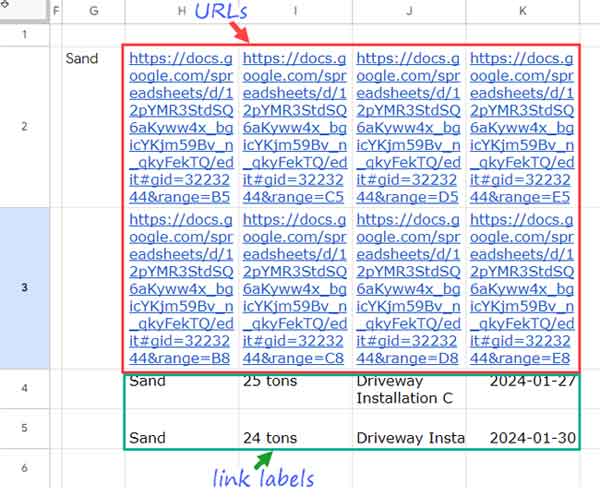
Where the Link Label is:

FILTER(f_range, c_rangeA=cA)

This is the second filter formula, which returns the values to use as link labels (the first filter formula returns the row numbers only).

That concludes how to use the HYPERLINK function with the FILTER function in Google Sheets.

Resources

Similar to using the HYPERLINK with the FILTER function, we can also use it with VLOOKUP, INDEX-MATCH, MIN, MAX, UNIQUE, etc. Here are those tutorials.

1. Search Value and Hyperlink Cell Found in Google Sheets
2. Create a Hyperlink to the Vlookup Output Cell in Google Sheets
3. UNIQUE Duplicate Hyperlinks in Google Sheets – Same Labels Different URLs
4. Two Ways to Hyperlink to an Email Address in Google Sheets
5. Hyperlink Max and Min Values in Column or Row in Google Sheets
6. Hyperlink to Index-Match Output in Google Sheets
7. Inserting Multiple Hyperlinks within a Cell in Google Sheets
8. Hyperlink to Jump to Current Date Cell in Google Sheets
9. Jump to the Last Cell with Data in a Column in Google Sheets (Hyperlink)
10. Hyperlink Calendar Dates to Events in Google Sheets