In this tutorial, let’s learn how to use Hyperlink to jump to the current date in a row or column in Google Sheets.
Dates are one of the most commonly appearing values in a table. It can be as a header row or a transaction column.
Whatever the data orientation, sometimes, we may want to quickly jump to the current date in a table.
The first solution that comes to our mind may be using Ctrl+F, the popular shortcut for search. But it has one issue!
What’s that?
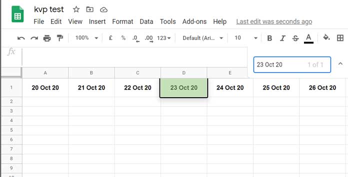
In the search field, we must type today’s date in the format that matches the date format in our table.
For example, my dates are in the format "dd mmm yy". I should make sure that I am using the same date format in the search field.
Further, there is a chance for forgetting the current date and using a wrong date to search.
We can solve this issues by creating a hyperlink formula to jump to current date in Google Sheets.
Introduction – Internal and External Hyperlinks
The Hyperlink function lets us create a hyperlink inside a cell. In basic form, it works like this.
For example, if you want to create a link to one of the pages on this blog, for example to the homepage, you can use the below formula in any cell.
=HYPERLINK("https://infoinspired.com","info inspired")If the formula is in cell A1, the formula would place the label “info inspired” in that cell.
Clicking on that label will take you to the homepage of this blog from your Google Sheets file.
The above is an example to external hyperlink (hyperlink to an external page) in Google Sheets.
What we want to do is to write a hyperlink formula to jump to the current date cell in Google Sheets. That means the hyperlink formula should link internally.
I mean the formula and the link would be in one sheet.
Here is an example of an internal hyperlink in Google Sheets.
I want to write a hyperlink formula in cell A1 that links to cell A10. If so, I should follow the below steps.
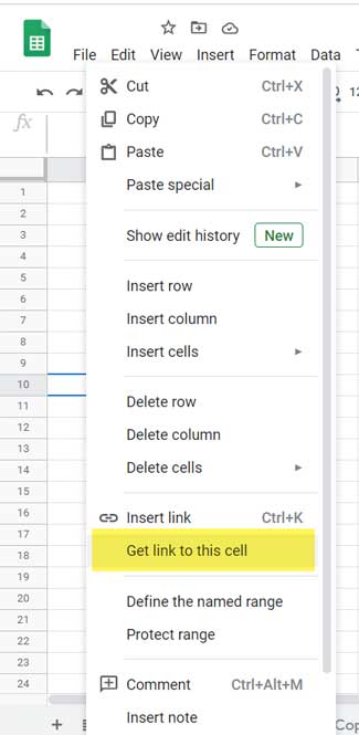
1. Right-click on cell A10 and from the shortcut menu, click the highlighted option “Get link to this cell”.
2. In cell A1, write the formula =HYPERLINK("URL_here","Link to A10") and replace URL_here with the just copied URL.
Note: The URL that you have copied in step # 1 is the URL of the cell A10. It would be something like this (take a special note at the cell address A10 at the end of the URL).
https://docs.google.com/spreadsheets/d/1KuDkBhmEZfm8-4kB9Tabcedfghijkl/edit#gid=1230788533&range=A10In order to create a hyperlink to jump to today’s date in Google Sheets, we should replace A10 in the URL with a dynamic formula that can return the cell address of the cell that contains the current date.
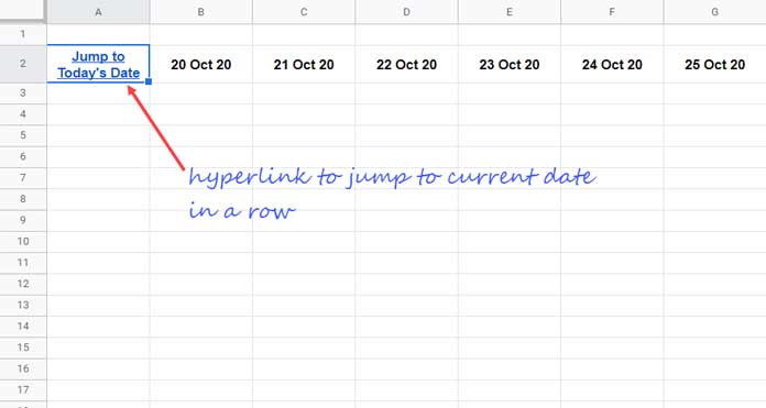
Hyperlink to Jump to Current Date in a Row
In the just above URL see the last part. It’s A10, the cell address of the copied URL.
The URL will be the same for all the cells in a sheet except the cell address at the end of the URL.
If the dates are in a row, we can use one simple formula to get the cell address of today’s date in that row.
Replacing A10 in the URL with that formula will be the solution to hyperlink to jump to the current date in a row in Google Sheets.
Steps
1. Get the URL of any cell in the current sheet as explained earlier.
2. Remove the cell address from the end of the URL.
3. In the below Generic Formula replace the URL_of_the_sheet with the URL you have in step 2 above.
=HYPERLINK("URL_of_the_sheet","Jump to Today's Date")It will look as below.
=HYPERLINK(
     "https://docs.google.com/spreadsheets/d/xxxxxx/edit#gid=352488775&range=",
     "Jump to Today's Date"
)
4. Add the below formula at the end of the URL.
&address(
     2,
     match(today(),B2:2,0)+1,
     4
)
Final Formula:
=HYPERLINK(
     "https://docs.google.com/spreadsheets/d/xxxxxx/edit#gid=352488775&range="&address(2,match(today(),B2:2,0)+1,4),
     "Jump to Today's Date"
)
The Address formula returns the cell ID of today’s date. How?
As you can see, the dates are in the range B2:G2. To make the range open, we can use B2:2 instead.
The Match formula, i.e. match(today(),B2:2,0), returns the relative column position (the counting starting from cell B2 to its right until today’s date) of the current date in this range.
To get the column number of this date, we must add the number 1 to this Match output as below.
match(today(),B2:2,0)+1Note: If the dates are in C2:2, then you should add 2 to the Match output.
I hope you could understand how to get column number from relative position.
In the Address function, if we input the row and column number, the formula would return the corresponding cell ID.
Syntax: ADDRESS(row, column, [absolute_relative_mode], [use_a1_notation], [sheet])
We know the dates are in the second row and we could find the column number using the above Match formula.
So the following formula would return the cell ID of the current date in the range B2:2.
address(2,match(today(),B2:2,0)+1,4)That’s all about hyperlink to jump to current date cell in a row in Google Sheets.
Hyperlink to Jump to Today’s Date in a Column
Here the steps 1, 2, and 3 are as per the above example. The one and only change that we want to make is in the Address formula.
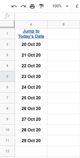
The dates are in A2:A11 or we can use open range A2:A. So we can use the below Match to find the relative row position of today’s date in A2:A.
match(today(),A2:A,0)To get the row number add 1 to this as the data is starting from the second row.
match(today(),A2:A,0)+1We know the dates are in the first column. So in Address, use 1 as the column number and the Match formula as the row number.
Here is the Address formula that you should add to the link as earlier.
&address(
     match(today(),A2:A,0)+1,
     1,
     4
)
As per the above example, hyperlink to jump to current date in a column, we can use the below formula.
=HYPERLINK(
     "https://docs.google.com/spreadsheets/d/xxxxxx/edit#gid=352488775&range="&address(match(today(),A2:A,0)+1,1,4),
     "Jump to Today's Date"
)
Can We Use a Timestamp Column?
If we use a timestamp column and create a hyperlink to jump to today’s date, we should slightly modify the Match part of the formula.
In Row Wise:
match(today(),arrayformula(int(A2:A)),0)In Column Wise:
match(today(),arrayformula(int(B2:2)),0)Here is my sample sheet. Don’t forget to replace the URL in the formula in the sample sheet. Otherwise, it will point to my original sheet, not the copy that you have just made.
Resources:
- How to Jump to Specific Sheet Tab in Google Sheets.
- Search Value and Hyperlink Cell Found in Google Sheets.
- Create a Hyperlink to Vlookup Output Cell in Google Sheets.
- UNIQUE Duplicate Hyperlinks in Google Sheets – Same Labels Different URLs.
- Hyperlink Max and Min Values in Column or Row in Google Sheets.
- Hyperlink to Index-Match Output in Google Sheets.
- Two Ways to Hyperlink to an Email Address in Google Sheets.
- Inserting Multiple Hyperlinks within a Cell in Google Sheets.


Thank you SO much! Every other guide out there uses a column to reference dates, but my sheet has the dates in a row like this one, so this is the only one that worked for me. THANK YOU!!
Excellent! Could this be adapted to find and jump to the word ‘Today’? For instance, if a cell contains the word ‘Today’ (e.g., A7), the cursor would jump to that cell. If A7 changes to blank and H4 now contains ‘Today,’ selecting the link would then jump to H4.
This could be done with a different formula. Let me check if I’ve already posted one (it’s hard to remember with over 1,250 posts). If not, I’ll try to write one.
Thanks for your patience! I’ve got a solution for you now. You can check it out in this post. Let me know if it works for your needs!
Hi, thank you for sharing your insights. However, I have a concern about the “Jump to Current Date Cell” hyperlink function in Google Sheets. I noticed that when I click on the hyperlink, it opens a new file tab.
Is there any way to revise the formula so that clicking on the link directly goes to the current date cell without opening up another identical file tab?
Make sure you are using the correct URL in the formula. If you would like me to test it, please share a sample sheet.
Okay, I understand. You are using a copy of my sample sheet. Please replace the URL in the formula with the new copied sheet’s URL.