There are two options to create a hyperlink to an email address in Google Sheets: using the HYPERLINK function or the Link command. Additionally, you can convert an email address into a People Chip.
You can make the email address clickable and open your email client to compose an email using either the HYPERLINK function or the Link command.
A People Chip is a feature that converts an email address into a chip displaying contact information, such as names and email addresses, in a visually distinct way within a cell.
While the Link menu command and the HYPERLINK function create clickable email addresses, People Chips require you to hover over the chip to view the contact information.
Create a Clickable Email Address with the Link Menu
This is the simplest method to make an email address clickable.
Steps:
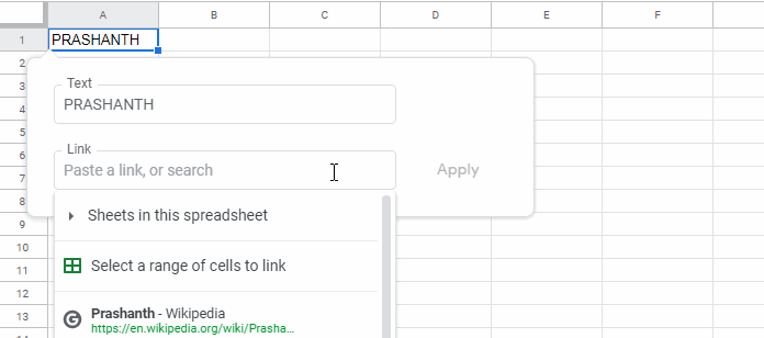
- Navigate to the cell where you want to create the clickable email address (e.g., cell A1).
- Go to the Insert menu and click on Link.
- In the first field labeled “Text”, enter the username (display text) or leave it blank.
- In the second field labeled “Paste a link, or search”, enter the email address you want to hyperlink.
- Click Apply.
Pros & Cons of the Link Command:
- Pros:
- Easy to create clickable links.
- Cons:
- Can only create one hyperlink at a time.
Create a Clickable Email Address Using the HYPERLINK Function
To hyperlink to an email address using a formula in Google Sheets, use the following syntax:
=HYPERLINK("mailto:[email protected]","username")Insert this formula into cell A1 or any empty cell. Replace [email protected] with the email address you want to hyperlink.
The “username” argument in the formula is the link label, which means the visible text in cell A1 will be “username”. Replace “username” with the actual username, such as “Prashanth”.
If you prefer the email address to appear as the link label instead of a name, use:
=HYPERLINK("mailto:[email protected]")Pros & Cons:
- Pros:
- Allows you to create multiple clickable email addresses at once.
- Cons:
- Requires familiarity with functions in Google Sheets. For instance, the argument separator in the formula is a comma, but in some locales, it may be a semi-colon.
Link Usernames in One Column to Email Addresses in Another Column
The HYPERLINK function works with the ARRAYFORMULA function, allowing you to convert a list of email addresses into clickable email addresses in one go.
Example:
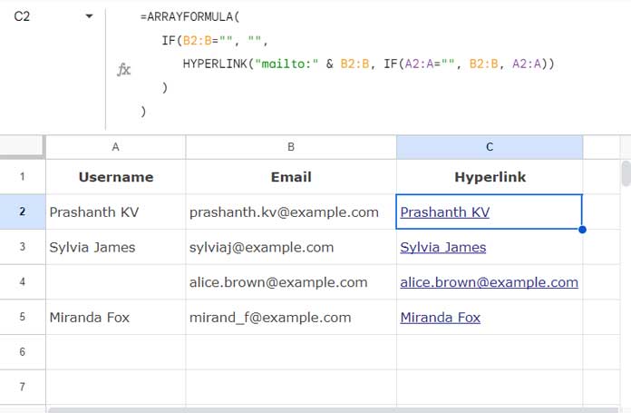
Column A has usernames, and column B has corresponding email addresses. The range is A1:B.
Insert the following formula in cell C2:
=ARRAYFORMULA(
   IF(B2:B="", "",
      HYPERLINK("mailto:" & B2:B, IF(A2:A="", B2:B, A2:A))
   )
)
If you do not want the usernames as the link label, you can leave column A blank.
Formula Breakdown:
The formula follows the IF function syntax IF(logical_expression, value_if_true, value_if_false):
logical_expression:B2:B=""– checks whether the email addresses are blank.value_if_true:""– returns an empty string if the logical expression evaluates to TRUE.value_if_false:HYPERLINK("mailto:" & B2:B, IF(A2:A="", B2:B, A2:A))
Breaking down the HYPERLINK formula:
The formula follows the HYPERLINK function syntax HYPERLINK(url, [link_label]):
url:"mailto:" & B2:B– creates a “mailto” link for each email address in column B.link_label:IF(A2:A="", B2:B, A2:A)– if the username is blank, use the email address as the link label; otherwise, use the username.
People Chips
To create a People Chip, navigate to the cell containing the email address and click Insert > Smart Chips > Convert to People Chip. This will only work with valid email addresses, meaning email addresses in your Google Contacts.
You can read more about this in the resources below.


Hi Prashanth,
I copied the array formula and got the message ‘invalid link,’ so I put the text in column B and the email address in column A, and it worked.
Hi, Herminia Mathieu,
Thank you for pointing out the error.
I have modified the formula within the post above from this-
=ArrayFormula(if(A1:A="",,HYPERLINK("mailto:"&A1:A,B1:B)))-to this.
=ArrayFormula(if(A1:A="",,HYPERLINK("mailto:"&B1:B,A1:A)))Prashanth-
I am racking my brain trying to figure out how to extract the email address from the hyperlinks in this spreadsheet. I have tried all sorts of scripts and REGEX formulas to no avail. Do you have any recommendations? Thank you for any advice you can offer. Kindly, Karen
Test Sheet: – link removed by admin –
Hi, Karen,
Please try this method.
https://infoinspired.com/google-docs/spreadsheet/extract-urls-in-google-sheets-without-script/