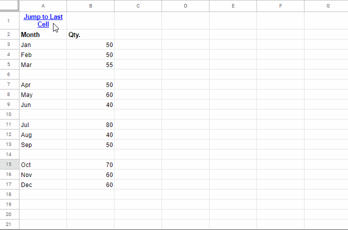
Using the keyboard shortcut Ctrl + ↓, we can jump to the cell just above the first blank cell in a column. But if you want to jump directly to the last cell with data in a column in Google Sheets, you can do it with a hyperlink.

The above shortcut works well if there are no blank cells between values. But when blank cells exist, you’ll need a formula-based solution.

In this Google Sheets tutorial, I’ll share two formula tips:

• How to create a hyperlink to jump to the last cell in a column
• How to create a hyperlink to jump to the last row in a table

Though they may sound similar, there’s a small but important difference. The first is about jumping to the last cell with data in a single column, while the second refers to jumping to the last row in a multi-column table.

Some people use Google Apps Script for these tasks, but we can do it with the built-in HYPERLINK function in Google Sheets.

Follow the steps below.

Hyperlink to Jump to the Last Cell with Data in a Column

Let’s start by creating a hyperlink (text or button) that jumps to the last non-blank cell in a column.

Steps:

1. In your sheet, click any cell—say, cell E3. Then right-click and select “View more cell actions > Get link to this cell.” You’ll see a notification saying, “Link copied to the clipboard”. That means the link to cell E3 is now saved.

2. Right-click on cell E3 again and choose Paste.

3. Remove the cell reference (E3) from the end of the pasted URL.
You’ll be left with just the base link to your sheet.

https://docs.google.com/spreadsheets/d/1YE3upO7UlY69r1wisVdD7eJjVt2UvIzqtYI1CCNAnns/edit#gid=1225485770&range=

4. Now, we need to find the cell address of the last non-blank cell in column A.
Use the following formula in cell E4 (as explained in my tutorial “Address of the Last Non-Empty Cell Ignoring Blanks in a Column in Excel”—which also applies to Sheets):

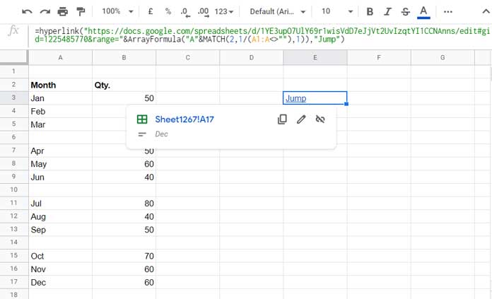
=ArrayFormula("A"&MATCH(2, 1/(A1:A<>""), 1))

5. Combine the base URL in E3 with the formula in E4 like this (you can do this in cell E3 itself):

="https://docs.google.com/spreadsheets/d/1YE3upO7UlY69r1wisVdD7eJjVt2UvIzqtYI1CCNAnns/edit#gid=1225485770&range="&ArrayFormula("A"&MATCH(2, 1/(A1:A<>""), 1))

After that, you can safely delete the formula in E4.

Note: Don’t copy the above URL—it’s from my sheet. Replace it with your sheet’s URL as shown in Step 1.

6. Now it’s time to create the actual hyperlink:

=HYPERLINK(
   "https://docs.google.com/spreadsheets/d/1YE3upO7UlY69r1wisVdD7eJjVt2UvIzqtYI1CCNAnns/edit#gid=1225485770&range="&ArrayFormula("A"&MATCH(2, 1/(A1:A<>""), 1)), 
   "Jump"
)

That’s it! This hyperlink will now jump to the last non-empty cell in column A.

Hyperlink Formula Note – Column A Limitation

You can place this formula in any column except column A. If you put it in column A, you’ll get a circular dependency error.

If you want to place the hyperlink in cell A1, we need to tweak the formula slightly:

Replace this:

ArrayFormula("A"&MATCH(2, 1/(A1:A<>""), 1))

With this:

ArrayFormula("A"&MATCH(2, 1/(A2:A<>""), 1)+1)

This change avoids referencing A1 directly and adjusts the MATCH result accordingly.

Then cut the formula from cell E3 and paste it into cell A1.

Tip: Feel free to change the hyperlink text "Jump" to any other label or even button-like characters such as 🔽, 🟧, etc.

For example:

=HYPERLINK(
   "https://docs.google.com/spreadsheets/d/1YE3upO7UlY69r1wisVdD7eJjVt2UvIzqtYI1CCNAnns/edit#gid=1225485770&range="&ArrayFormula("A"&MATCH(2, 1/(A2:A<>""), 1)+1), 
   "🔽"
)

To remove the underline from the hyperlink (which appears by default), just press Ctrl + U on the cell.

Hyperlink to Jump to the Last Row of a Table

So far, we’ve learned to jump to the last cell with data in a column. But what if you want to jump to the last row in a table?

Let’s say your table is in the range A2:B17, but cells A16 and A17 are blank. The previous formula would take you to A15.

That’s fine if you’re only concerned with column A. But if you’re considering the full table (A2:B17), it’s not ideal.

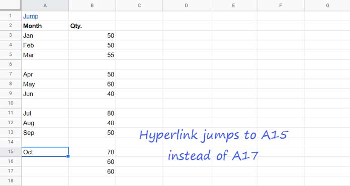
Issue in Linking to the Last Row of a Table

To fix this, we just need to combine the values of both columns in the formula.

Here’s the updated formula:

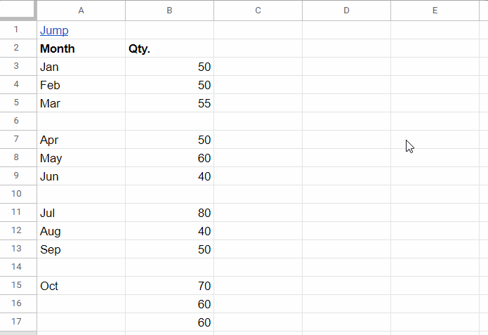
=HYPERLINK(
   "https://docs.google.com/spreadsheets/d/1YE3upO7UlY69r1wisVdD7eJjVt2UvIzqtYI1CCNAnns/edit#gid=1225485770&range="&ArrayFormula("A"&MATCH(2, 1/(A2:A&B2:B<>""), 1)), 
   "Jump"
)

We simply changed A2:A to A2:A&B2:B—this treats a row as blank only if both cells in columns A and B are empty.

Hyperlink to Jump to the Last Row of a Table – More Columns?

If your table has more than two columns, no worries.

Just combine more ranges using the ampersand. For example, if your table spans columns A to D, use:

A2:A&B2:B&C2:C&D2:D

That’s all about how to jump to the last cell or row with data in a column or table in Google Sheets.

Thanks for the stay. Enjoy!

Resources

• Search for a Value and Hyperlink the Found Cell in Google Sheets
• Hyperlink to VLOOKUP Result in Google Sheets (Dynamic Link)
• Hyperlink Max and Min Values in Column or Row in Google Sheets
• Hyperlink to Index-Match Output in Google Sheets
• How to Create a Hyperlink to an Email Address in Google Sheets
• Insert Multiple Hyperlinks within a Cell in Google Sheets
• Hyperlink to Jump to Current Date Cell in Google Sheets
• Find the Address of the Last Used Cell in Google Sheets