This tutorial on finding the cell address of the last non-empty cell, while ignoring blanks in a column, applies to both Excel and Google Sheets.

To prevent any confusion, I intentionally excluded Google Sheets from the title. Allow me to clarify why.

Previously, I authored a Google Sheets tutorial covering the same topic on this site titled “Find the Cell Address of a Last Used Cell in Google Sheets.”

Upon further reflection, I discovered a more efficient method for finding the cell address of the last non-empty cell, ignoring blanks in a column in both Excel and Google Sheets.

Now faced with two options:

1. Revise the original tutorial to incorporate the new formula.
2. Create a new tutorial that applies to both Excel and Google Sheets, then update the original tutorial with a link to the new one.

I chose the latter. Even though Google Sheets is not explicitly mentioned in this tutorial, please be aware that the formula can also be applied to Google Sheets. So, let’s proceed.

How to Find the Address of the Last Non-Empty Cell Ignoring Blanks in a Column in Excel

First, let’s understand the concept of finding the last non-empty cell in a column, ignoring blank cells. The screenshot below illustrates this:

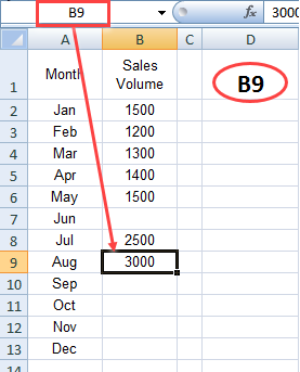
In this example, the target column is B. Within column B, the last non-empty cell, excluding blanks, is cell B9.

Cell B7 is blank, and we want to skip that and directly identify the last non-empty cell, returning its address.

Here is the formula to achieve this in Excel. Enter this as an array formula in Excel:

="B"&MATCH(2, 1/(B:B<>""), 1)

How to Use the Formula in Excel:

For Older Versions of Excel:

1. Copy and paste the formula into the formula bar in Excel (use any blank cell other than column B).
2. Use the keyboard shortcut Ctrl+Shift+Enter to turn it into an array formula.

For Excel Versions that Support Dynamic Arrays:

• Simply insert the formula into any blank cell other than column B.

Now, for Google Sheets users, here is the equivalent formula:

=ArrayFormula("B"&MATCH(2, 1/(B:B<>""), 1))

Retrieve the Cell Address of the Last Non-Blank Cell, Ignoring Blanks in Excel: Formula Breakdown

Step-by-Step Instructions:

Step 1:

Type the following formula in cell D1:

=B1<>""

This formula will return TRUE in cell D1. To test it, delete the value in cell B1, and the formula will then return FALSE.

Note: In Excel/Sheets, TRUE is equal to the number 1, and FALSE is equal to the value 0.

Step 2:

Modify the formula from Step 1 as follows:

=1/(B1<>"")

This means if there is a value in cell B1, the formula is equal to 1/1; otherwise, it’s 1/0, resulting in either 1 or #DIV/0!.

Step 3:

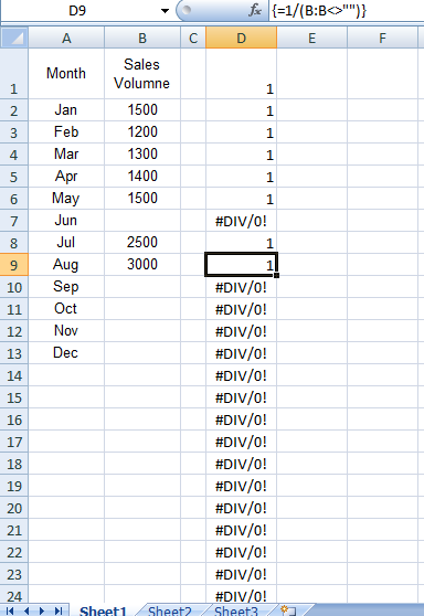
Select the entire column D and modify the formula as below:

=1/(B:B<>"")

This formula must be entered as an Array Formula in the older versions of Excel. The result will show 1 in all cells with values in column B, or an error. The last value in column D is in the 9th row.

Step 4:

Utilizing the MATCH function, return the row number (9). In any blank cell, enter the following formula and press Ctrl+Shift+Enter:

=MATCH(2, 1/(B:B<>""), 1)

Delete the formula and the output in column D, as they were used for the step-by-step explanation.

Step 5:

Now, having determined the row number of the last non-empty cell in a column, ignoring blanks in Excel, convert this row number to a cell address by combining the column letter with the row number.

="B"&MATCH(2, 1/(B:B<>""), 1)

Conclusion

In summary, we can employ the MATCH function to find the cell ID of the last used cell in Excel.

In our formula, we’ve hardcoded the column letter. If desired, you can utilize the ADDRESS function with the Step 4 formula to find the cell ID without hardcoding the column letter. Here’s the revised formula:

=ADDRESS(MATCH(2, 1/(B:B<>""), 1), COLUMN(B:B))

That concludes the tutorial. Thank you for your attention. Enjoy!