Find everything you need to know about VLOOKUP in Max Rows in Google Sheets right here. You can customize VLOOKUP to return values specifically from the max rows in Google Sheets.

Many spreadsheet-related tasks rely on VLOOKUP in one way or another, although XLOOKUP is gradually gaining popularity. Mastering VLOOKUP in all its variations will give you an edge in data manipulation.

This Google Sheets tutorial covers the following points:

1. Find the maximum value in a column and return the corresponding value from the next column.
2. Look up a search key (possibly a string) and return either the maximum value or a value from the row containing the maximum value. This involves handling cases where the search key appears multiple times in the search column, but we only want the maximum value or a value associated with that row.

These two use cases are what I refer to as “VLOOKUP in Max Value Rows.”

1. Find Max Value and Return Value from Corresponding Row

This is an example of using the MAX function with the VLOOKUP function in Google Sheets.

For this type of lookup, you can combine the MAX function with VLOOKUP. Instead of directly providing a search key in VLOOKUP, use the MAX function to return the maximum value as the search key. Here’s an example:

=VLOOKUP(MAX(A2:A9), A2:B9, 2, FALSE)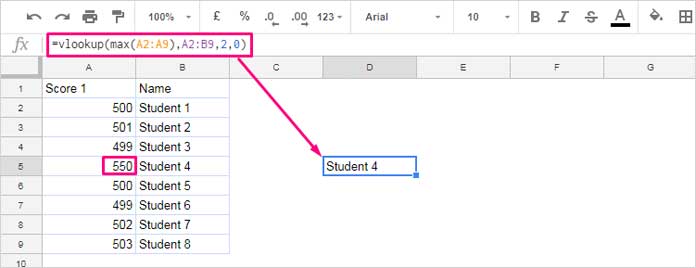

In this formula, the search key is the maximum value in the range A2:A9, returned by the MAX function. VLOOKUP searches for this value in the range A2:A9 and returns the corresponding value from the next column.

In most cases, the column containing the max value will be the second, third, or fourth column. If that’s the case, you should rearrange the table in the VLOOKUP function so that the search column is the first column.

For example, if the name column is the first column and the score column is the second, use the following formula:

=VLOOKUP(MAX(B2:B9), {B2:B9, A2:A9}, 2, FALSE)

Related: Reverse Vlookup Examples in Google Sheets [Formula Options]

The above examples demonstrate how to use VLOOKUP with max rows in Google Sheets. Now, let’s move on to a completely different scenario.

Note: If there are multiple max values, the formula will return the value corresponding to the first one. If you want all the values, you should use the FILTER function instead.

2. VLOOKUP a Search Key and Return Max Value

This is an example of using the VLOOKUP function with the SORT function in Google Sheets.

In this case, the search key is not the max value, so you don’t need to use the MAX function to find it. You already have a search key, which can be any value, possibly a text string.

What you want to do is search for this value in the search column and return the corresponding value from the first found row. If the search key appears multiple times, to get the max value, we will sort the range by the VLOOKUP index column (the result column) in descending order.

This is what’s known as “VLOOKUP in max value rows” in Google Sheets. Here’s an example:

The following formula searches for “Student 2” in column A and returns their max score from column B:

=VLOOKUP("Student 2", SORT(A2:B9, 2, FALSE), 2, FALSE)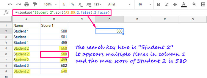

In this example, I’ve sorted the VLOOKUP range by the result column (i.e., score) in descending order.

Without using SORT, the VLOOKUP formula would return the value 550 from cell B5, because “Student 2” first appears in that row. However, by sorting the data range in descending order based on column B, the max values are moved to the top. So, the max value (from row #6) will now appear at the top, replacing the value from row #5.

Similar to using MAX with VLOOKUP, if the search key is not in the first column of the range, you can virtually make it the first column by using curly braces.

Additional Tips

VLOOKUP in Max Rows and Multiple Search Keys

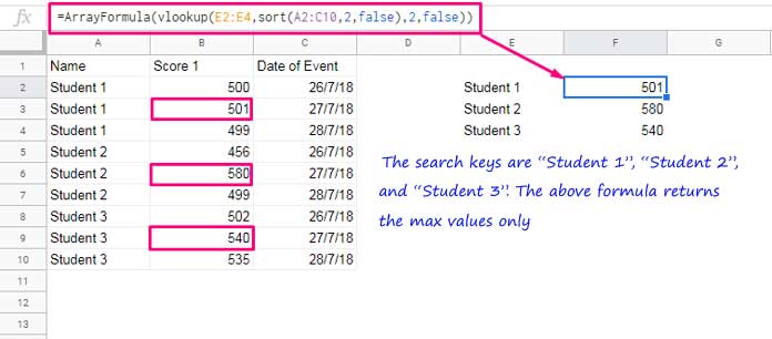
In the example above, there is only one search key. If you want to look up multiple values from only the max value rows, you can use ARRAYFORMULA with VLOOKUP as follows:

=ARRAYFORMULA(VLOOKUP(E2:E4, SORT(A2:C10, 2, FALSE), 2, FALSE))

This formula searches for the keys in E2:E4 in the sorted range A2:C10 and returns the value from the second column. The sorting places the max values at the top, so VLOOKUP returns the results from the max value rows only.

VLOOKUP Alternative to Return Values from Max Rows

You can replace VLOOKUP with SORTN to return values from the max value rows.

Similar to VLOOKUP, you must first sort the range by the result column in descending order. In this case, it’s SORT(A2:C10, 2, FALSE), which is similar to how VLOOKUP works.

Then, instead of VLOOKUP, we will use the SORTN function. The role of this function here is to keep only the top row of each item based on the search key column.

Here’s the formula:

=SORTN(SORT(A2:C10, 2, FALSE), 9^9, 2, 1, TRUE)

Where:

• 9^9 is the maximum number of rows in the result. This is an arbitrarily large number, and you can specify any number you like.
• 2 refers to the display_ties_mode in SORTN to remove duplicates. Here, it helps retain the top rows (the max value rows).
• 1 is the column index based on which the duplicates are determined.
• TRUE sets the sort order.

Resources

• Find Min, Max in a Matrix and Return a Value from the Same Row
• Removing Duplicates In Google Sheets: Built-In Tool & Formulas
• How to Find Max Value in Each Row in Google Sheets
• Highlight Max Value Leaving Duplicates in Row Wise in Google Sheets
• VLOOKUP – Find a Search Key in Multiple Columns (Matrix) in Google Sheets