An exact match in Google Sheets database functions means fully matching the criterion, not partially, in the criteria field.
It’s a simple but important concept, as it directly impacts the output of database functions.
You might wonder why this is so important. Let me explain.
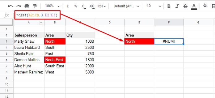
Take the DGET function, for example. Multiple occurrences of similar conditions can prevent it from working properly. If your criterion is “North,” and the criteria column contains both “North” and “North East,” DGET will return an error due to the partial match of “North” within “North East.” Because “North East” starts with “North”.
In other database functions, using the same criteria will result in incorrect results, although they won’t return an error.
However, you won’t face this issue when using numeric or date values as criteria.
Let’s explore how to apply exact match criteria in Google Sheets’ database functions (applicable to all functions listed in the Resources at the bottom).
Using Exact Match Criteria from Cell References in Database Functions
To ensure an exact match in database functions, place an equal sign before the criterion.
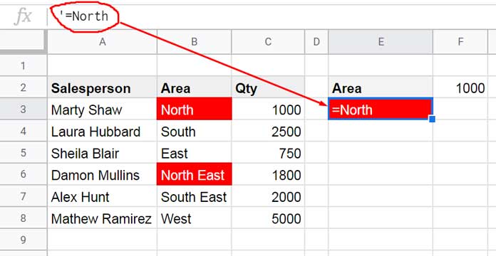
For example, to match North, you should specify it as =North. However, entering this directly in a cell will return a #NAME? error, as Google Sheets will interpret “North” as a named range that doesn’t exist.
To avoid this, precede the equal sign with an apostrophe. Enter the criterion as '=North.
Example:
Assume your database is in the range A2:C8, where A2:C2 contains “Salesperson,” “Area,” and “Qty.”
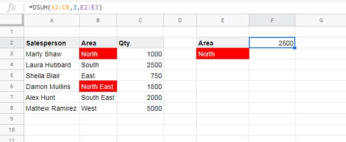
Enter the criteria in E2:E3, with E2 containing Area and E3 containing '=North.
In cell F2, use the following formula to search the criteria in the database and return the corresponding value from the third column:
=DGET(A2:C8, 3, E2:E3)Syntax: DGET(database, field, criteria)
How to Hardcode Exact Match Criteria in DB Functions
When hardcoding the criteria, you shouldn’t include the apostrophe for an exact match. You can rewrite the formula as follows:
=DGET(A2:C8, 3, {"Area"; "=North"})For more information on using criteria, check out Mastering Criteria in Database Functions in Google Sheets.
Resources
New to database functions? The following tutorials cover all of them:


Thanks, Prashanth.
I was hoping to avoid using the
=in front of the criteria as it looks a bit confusing to others, but seems like I’m stuck with that!I did find a tip to work around it though, which I’ll share in case anyone else looks at this thread. I changed the font color of the
=to white to make it invisible. 🙂Hi, Deborah Kragten,
I would rather prefer the below method.
The criterion in E2:
NorthFormula:
=dsum(A1:C5,3,{E1;"="&E2})Instead of;
The criterion in E2:
=NorthFormula:
=dsum(A1:C5,3,E1:E2)This is really helpful thanks.
In your DSUM example above;
=DSUM(A2:C8,3,{"Area";"=North"})what if I want to use a cell reference instead of “=North” so that I can copy the formula down. In your example, Col E might have North, South, and West under Area with the formula then copied down from F2.
I initially used just the cell ref in the normal way, then ran into the problem of it summing non-exact matches as you describe. my formula:
=dsum('Transactions'!$A$3:$J$255,10,{"Ref";$B45})I’d like to hardcode the exact match functionality into the formula so I don’t have to put an apostrophe and equals in front of my data.
Thanks!
Hi, Deborah,
Good question 🙂
The criterion must any way entered with
=sign as shown on the image under the title ‘Criteria as Cell Reference in DGET’.Assume the criteria are in E3, E4, E5, and so on and the field label of the criteria is in E2.
So when dragging the formula from F2, the field label E2 in the formula must be absolute, i.e.
$E$2, and criterion E3 in the formula must be relative, i.e.$E3.Here is that DSUM exact match formula with drag-drop criterion reference.
=DSUM($A$2:$C$8,3,{$E$2;$E3})When you drag this DSUM formula down, it picks the criterion from the rows down.