The DPRODUCT function in Google Sheets multiplies the values in a specified numeric field in a table matching conditions.
While less commonly used in real-life scenarios, real-life examples of its application are rare to find even with extensive searching. Nonetheless, DPRODUCT remains invaluable for conducting conditional product calculations within structured datasets.
This tutorial explains how to use the DPRODUCT function with a real-life example.
As a side note, database functions work only with structured data, a data set with field labels (header row with labels), and no merged cells.
If you have such data and are not well-versed in functions to conditionally return a product, then DPRODUCT is your best bet.
DPRODUCT Function: Syntax and Arguments
Syntax:
DPRODUCT(database, field, criteria)The DPRODUCT function has three arguments as per the syntax, and here is what they represent.
Arguments:
database: The structured table to consider. Each column in the table must contain a label in the top row, usually representing the data in the column.field: Indicates the column in which to apply the product calculation. You can specify the column number (the first column will be numbered one) or the field label.criteria: An array or range containing the conditions to apply filtering before product calculation.
Example of Using the DPRODUCT Function in Google Sheets
Assume you are awarded a job to install HT Panels and Lighting Poles amounting to USD 80,000. You will receive the payment as per the billing break-up approved.
This means each payment will be released upon the completion stage at the site, such as mobilization, supply of material, installation, testing, and commissioning.
Sample Data:
| Item | Qty (Nos) | Payment Stage | Payment Percentage/Amount |
| HT Panel | 4 | Total | $20,000.00 |
| HT Panel | 4 | Mobilization | 5% |
| HT Panel | 4 | Supply of Material | 40% |
| HT Panel | 4 | Installation | 40% |
| HT Panel | 4 | Testing | 10% |
| HT Panel | 4 | Commissioning | 5% |
| Lighting Poles | 100 | Total | $60,000.00 |
| Lighting Poles | 100 | Mobilisation | 5% |
| Lighting Poles | 100 | Supply of Material | 60% |
| Lighting Poles | 100 | Installation | 20% |
| Lighting Poles | 100 | Testing | 10% |
| Lighting Poles | 100 | Commissioning | 5% |
Assume you want to calculate the amount you get after supplying the Lighting Poles. Here we can use the DPRODUCT function in Google Sheets.
Let’s arrange the sample data and criteria range for the explanation.
Sample Data and Criteria Arrangement for the DPRODUCT Function
Sample Data Preparation:
Copy and paste the table above into an empty sheet of a Google Sheets file. Leave 4 blank rows above for spacing. So, the range here will be A5:D17.
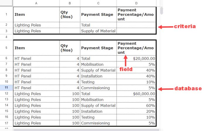
Criteria Preparation:
- In A1:D1, copy and paste the header of the table.
- In C2:C3, under the field ‘Payment Stage’, enter “Total” and “Supply of Material”.
- Under the field ‘Item’ in A2:A3, enter “Lighting Poles”.
This means we need to find the product of values in the filtered rows where A5:D17 matches “Lighting Poles” and C5:C7 matches either “Total” or “Supply of Material”.
We have properly arranged the database and criteria for the DPRODUCT function. Now coding the formula is just easy.
Formula:
=DPRODUCT(A5:D17, "Payment Percentage/Amount", A1:D3)Where:
database–A5:D17field–"Payment Percentage/Amount"criteria–A1:D3
Replace “Supply of Material” in cell C3 with “Installation”. The DPRODUCT will return the installation amount of Lighting Poles.
Alternatives to the DPRODUCT Function in Google Sheets
If your data lacks structure, consider using a combination of FILTER + PRODUCT, SUMPRODUCT, or QUERY to calculate conditional products.
Unlike DPRODUCT, these functions may become complex depending on the number of criteria you want to apply.
The benefit is that they will likely work well with both structured and unstructured data, provided there are no merged cells in the range.
For example, we can replace our previous DPRODUCT formula with this FILTER and PRODUCT combo:
=PRODUCT(FILTER(D6:D17, (A6:A17="Lighting Poles")*((C6:C17="Total")+(C6:C17="Supply of Material"))))


