With a simple workaround, you can use DGET as an array formula with single or multiple criteria in Google Sheets. This means you can look up the values for multiple search keys in one go—no need to write multiple DGET formulas manually. Better yet, it supports multiple criteria, allowing you to match values from more than one column.
The easiest method uses the MAP + LAMBDA combo, but we’ll also cover a solution that works without LAMBDA.
Why DGET Doesn’t Work with ArrayFormula
The DGET function is used to search for a record in a database that meets specific criteria and returns a value from a specified field.
Syntax:
DGET(database, field, criteria)The issue? DGET is designed to return a single value from a single column (field) for one matching record. If there are multiple matches in the database or if you try to expand it using ArrayFormula over multiple search keys, it will throw a #NUM! error because DGET expects only one match at a time.
Example:
=DGET($A$1:$E, "Maths", {"First Name"; G2})This works with a single search key in cell G2. But what happens if you try to expand it like this?
=ArrayFormula(DGET($A$1:$E, "Maths", {"First Name"; G2:G}))You’ll get a #NUM! error:
More than one match found in DGET evaluation.
Even with multiple criteria like:
=DGET($A$1:$E, "Maths", {"First Name", "Last Name"; G2, H2})It works fine for one row. But this fails:
=ArrayFormula(DGET($A$1:$E, "Maths", {"First Name", "Last Name"; G2:G, H2:H}))So how can we work around this? Let’s explore two methods to create a DGET Array Formula that works down a column.
Sample Data
Here’s the dataset we’ll use:
| First Name | Last Name | Maths | Physics | Chemistry |
|---|---|---|---|---|
| Rita | Webb | 90 | 92 | 91 |
| Eric | Reeves | 92 | 95 | 91 |
| Kristine | Sanchez | 95 | 85 | 79 |
| Donna | Reeves | 79 | 90 | 85 |
| Paula | Hopkins | 70 | 91 | 84 |
| Joan | Garcia | 80 | 70 | 90 |
| Alton | Moss | 85 | 86 | 92 |
Method 1: DGET Array Formula Without LAMBDA
Let’s say you want to look up the “Maths” marks for Rita, Paula, and Joan in one go using a DGET array formula.
We’ll use the fact that DGET accepts field labels (e.g., “Maths”) instead of just column indexes. To make it work with an array formula, we’ll use the TRANSPOSE function to change the layout of our data.
1. Lookup Using a Single Criteria Column
Formula:
=ArrayFormula(IFERROR(DGET(TRANSPOSE(A1:E), G2:G, {"First Name"; "Maths"})))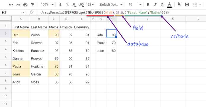
Explanation:
TRANSPOSE(A1:E)turns the database sideways (please refer to the image below).G2:Gcontains the list of names (“Rita”, “Paula”, etc.).- The criteria range
{"First Name"; "Maths"}swaps places: “First Name” becomes the lookup field and “Maths” becomes the value we’re extracting.
Tip: Change the Column You’re Extracting From
To get values from another subject column (say, “Chemistry”), just replace "Maths" with "Chemistry" in the formula.
2. Lookup Using Multiple Criteria Columns (First Name + Last Name)
When you need to use two criteria columns, such as “First Name” and “Last Name”, follow this pattern:
Formula:
=ArrayFormula(IFERROR(DGET(TRANSPOSE({A1:A&" "&B1:B, C1:E}), G2:G&" "&H2:H, {"First Name Last Name"; "Maths"})))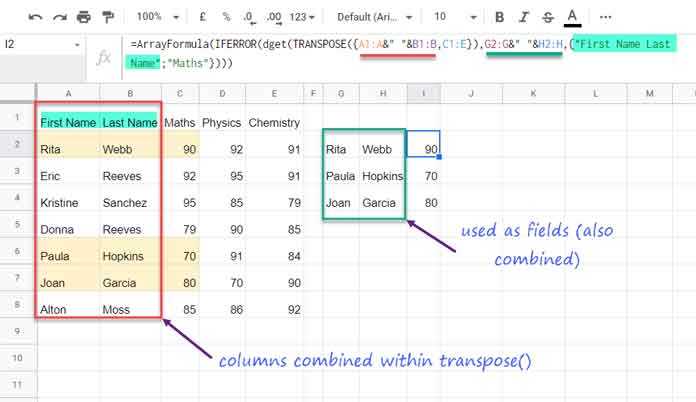
Explanation:
{A1:A&" "&B1:B, C1:E}combines “First Name” and “Last Name” columns into a single string and appends the remaining columns.G2:G&" "&H2:His the combined search key from two columns.{"First Name Last Name"; "Maths"}is the criteria: search this full name and return the “Maths” score.
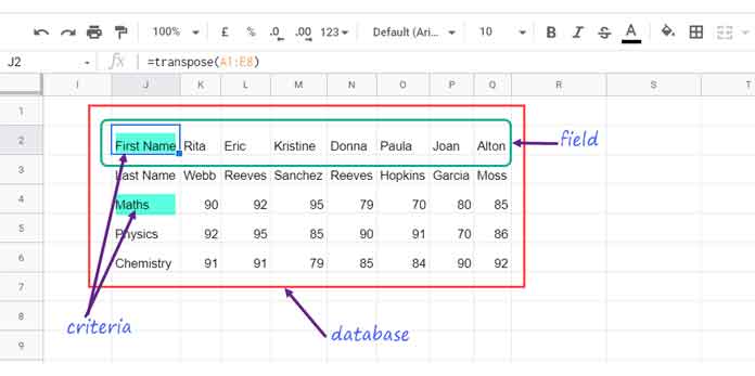
Preview Your Transposed Range (Optional):
To better visualize how the database is transformed:
=ArrayFormula(TRANSPOSE({A1:A8&" "&B1:B8, C1:E8}))Method 2: DGET Array Formula with LAMBDA
For a cleaner and more scalable approach, especially when using multiple lookup values, you can use the MAP + LAMBDA combo.
1. Lookup Using a Single Criteria Column
Let’s say you have:
"First Name"inG1- Search keys (names) in
G2:G4
Then use this formula in H2:
=MAP(G2:G4, LAMBDA(x, DGET(A1:E, 3, {G1; x})))This will return a column of Maths scores (assuming “Maths” is the 3rd column).

2. Lookup Using Multiple Criteria Columns
If you want to search using both “First Name” and “Last Name”, do the following:
- Enter
"First Name"inG1,"Last Name"inH1 - Put search values below each (e.g., names in
G2:G4andH2:H4) - Then use this in
I2:
=MAP(G2:G4, H2:H4, LAMBDA(x, y, DGET(A1:E, 3, {G1, H1; x, y})))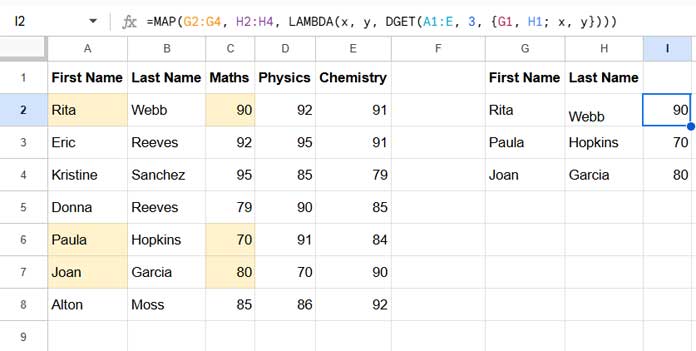
Advantages of the LAMBDA Approach Over TRANSPOSE
While both methods allow you to perform DGET-style lookups for multiple search keys, the LAMBDA approach—especially when combined with MAP—offers several distinct advantages:
1. Easier to Read and Maintain
The LAMBDA approach keeps your formula logic clean and readable:
- No need to transpose the database.
- No complicated reshaping of data or combining fields.
- Each search key is processed in its own row, making debugging and editing much simpler.
Example (single field):
=MAP(G2:G4, LAMBDA(x, DGET(A1:E, 3, {G1; x})))Compare that to the TRANSPOSE-based version, which requires flipping the data and reversing the field-criteria roles—a clever but less intuitive trick.
2. Works with Multiple Fields and Multiple Criteria
Another key advantage is that LAMBDA lets you return multiple column values in a single go—even when using multiple search criteria.
For example, this formula returns both “Maths” and “Physics” scores for each student:
=ArrayFormula(MAP(G2:G4, H2:H4, LAMBDA(x, y, DGET(A1:E, {3, 4}, {G1, H1; x, y}))))This is not possible with the TRANSPOSE-based method, which can only return a single value at a time.
Why this matters:
- You can look up by both “First Name” and “Last Name” and return scores from multiple subjects.
- The result expands across columns, delivering structured, multi-value output with minimal formula complexity.
Which Method Should You Use?
- Use the non-LAMBDA method if your dataset is very large and the LAMBDA approach becomes slow or fails to perform reliably.
- Use the MAP + LAMBDA method for cleaner, more flexible formulas that automatically expand down a column.
Both methods give you a way to scale DGET—something it wasn’t originally designed for.


