This post is all about using NOT in REGEXMATCH in Google Sheets.
Sometimes, instead of using NOT in REGEXMATCH in Google Sheets, you may prefer alternatives like FIND or SEARCH, depending on whether you need case-sensitive or case-insensitive matching. In this post, I’ll show you how to apply NOT in REGEXMATCH and also how to achieve the same result using FIND (case-sensitive) and SEARCH (case-insensitive).
Learning RE2 regular expressions and how they work in Google Sheets is not as hard as you may think. The best way is to start with simple examples — you can also check out my detailed REGEXMATCH tutorial.
How to Use NOT in REGEXMATCH in Google Sheets
Google Sheets doesn’t support advanced negative lookahead expressions like (?!...). So, you can’t directly negate text within the regex itself. It intentionally omits advanced features that could cause security vulnerabilities or excessive processing time.
The alternate way is to use the NOT logical operator along with REGEXMATCH in Google Sheets.
Assume I want to check whether cell D25 doesn’t contain the word "inspiration."
The below formula in any other cell will do the test and return TRUE or FALSE Boolean values.
Formula 1 (case-insensitive):
=NOT(REGEXMATCH(D25, "(?i)inspiration"))If it returns TRUE, it means "inspiration" is not present in D25.
Formula 2 (case-sensitive):
=NOT(REGEXMATCH(D25, "inspiration"))Alternatives Using NOT with FIND and SEARCH
The above two formulas show how to use NOT in REGEXMATCH in Google Sheets. But if you’d rather avoid regular expressions, you can use SEARCH (case-insensitive) or FIND (case-sensitive).
Case-insensitive (SEARCH):
=NOT(IFERROR(SEARCH("inspiration", D25)))Case-sensitive (FIND):
=NOT(IFERROR(FIND("inspiration", D25)))How do these formulas work?
- FIND/SEARCH return the position of the word in D25 if found.
- If the word is not found, they throw a
#VALUE!error. - IFERROR catches that error and turns it into a blank (
""). In Google Sheets, a blank is treated as FALSE. - Finally, wrapping it in NOT flips the logic, giving you TRUE when
"inspiration"is not found.
NOT in REGEXMATCH Array Formulas in Google Sheets
You can easily extend these formulas to work over a range using ARRAYFORMULA.
For example, across D25:D28:
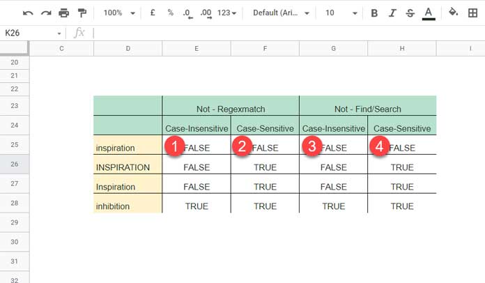
E25 (case-insensitive REGEXMATCH):
=ArrayFormula(NOT(REGEXMATCH(D25:D28, "(?i)inspiration")))F25 (case-sensitive REGEXMATCH):
=ArrayFormula(NOT(REGEXMATCH(D25:D28, "inspiration")))G25 (SEARCH alternative):
=ArrayFormula(NOT(IFERROR(SEARCH("inspiration", D25:D28))))H25 (FIND alternative):
=ArrayFormula(NOT(IFERROR(FIND("inspiration", D25:D28))))Match and NOT Match in a Single Formula in Google Sheets
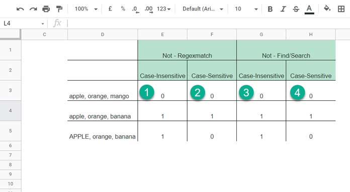
What if you want to test both conditions in the same formula? For example, check if "apple" is present and "mango" is not present in D3.
Using REGEXMATCH:
Case-insensitive:
=REGEXMATCH(D3, "(?i)apple")*NOT(REGEXMATCH(D3, "(?i)mango"))Case-sensitive:
=REGEXMATCH(D3, "apple")*NOT(REGEXMATCH(D3, "mango"))Using SEARCH/FIND alternatives:
Case-insensitive:
=LEN(IFERROR(SEARCH("apple", D3)))*NOT(LEN(IFERROR(SEARCH("mango", D3))))Case-sensitive:
=LEN(IFERROR(FIND("apple", D3)))*NOT(LEN(IFERROR(FIND("mango", D3))))👉 Note: These formulas return 1 (TRUE) or 0 (FALSE). You can wrap them with =IF(..., TRUE, FALSE) if you want explicit Boolean values.
And yes, these also work with ARRAYFORMULA over a range!
Conclusion
Using NOT in REGEXMATCH in Google Sheets is the most straightforward way to check whether a cell does not contain a specific word or phrase. Since Google Sheets doesn’t support advanced negative lookaheads, the trick is to wrap REGEXMATCH with the NOT function.
If you prefer, you can achieve the same result using FIND (case-sensitive) or SEARCH (case-insensitive). Both approaches are simple, flexible, and can also be expanded into array formulas for checking entire ranges at once.
Choose REGEXMATCH when you need the power of regular expressions, and FIND/SEARCH when you want lightweight alternatives.
Resources
- REGEXMATCH in FILTER Criteria in Google Sheets [Examples]
- Match Two Columns with Values in Any Order Using REGEXMATCH
- REGEXMATCH in SUMIFS and Multiple Criteria Columns in Google Sheets
- REGEXMATCH Dates in Google Sheets – Single/Multiple Match
- How to Use REGEXMATCH in AVERAGEIF in Google Sheets
- Case-Insensitive REGEXMATCH in Google Sheets (Partial or Whole)


