You can filter data based on a list in another tab in Google Sheets using the FILTER function combined with the XMATCH function. This approach allows you to dynamically extract data that matches a predefined list of criteria from another sheet.
Generic Formula:
=FILTER(range, XMATCH(criteria_range, list)) For example, the following formula filters the range A2:B in Sheet1 based on a list of items in A2:A5 in Sheet2:
=FILTER(Sheet1!A2:B, XMATCH(Sheet1!A2:A, Sheet2!A2:A5)) This formula matches the items in A2:A of Sheet1 with the list in A2:A5 of Sheet2.
Example: Filter Data Based on a List in Another Tab
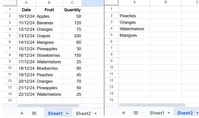
The sample data includes the date, fruit names, and quantity in the range A1:C of Sheet1, with headers in row 1. The filter range is A2:C, and the criteria range is the list in A2:A5 of Sheet2.
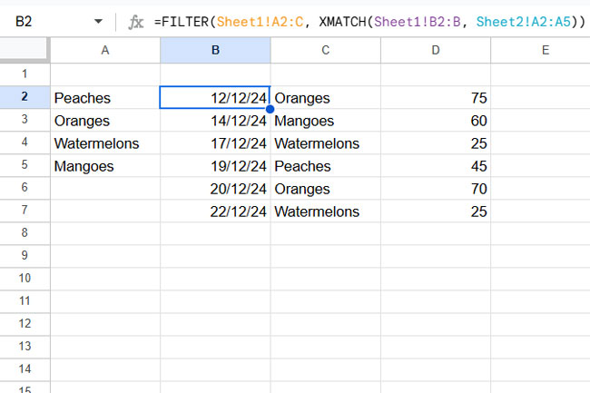
To filter this range based on a list of fruit names in A2:A5 from Sheet2, use this formula:
=FILTER(Sheet1!A2:C, XMATCH(Sheet1!B2:B, Sheet2!A2:A5))This formula works seamlessly to filter data based on a list in another tab. You can insert it in either Sheet1 or Sheet2.
Common Errors to Watch Out For:
- #N/A:
- This error occurs if the list is empty or the values in the list do not match the column being filtered (e.g.,
B2:BinSheet1). - Double-check that you’re referencing the correct columns and that the list in
Sheet2contains relevant values.
- This error occurs if the list is empty or the values in the list do not match the column being filtered (e.g.,
- #REF!:
- This error means the formula cannot expand because of pre-existing values in the output cells.
- Ensure there is enough empty space to display the filtered results.
The combination of FILTER and XMATCH is the easiest way to filter data based on a list in another tab. If you need case-sensitive filtering, you can replace the XMATCH function with REGEXMATCH, as described below.
Formula Explanation
FILTER Function Syntax:
FILTER(range, condition1, [condition2, …]) - range: The data to filter (
Sheet1!A2:Cin this case). - condition1: The filter condition (
XMATCH(Sheet1!B2:B, Sheet2!A2:A5)).
XMATCH Function:
The XMATCH function checks whether each value in Sheet1!B2:B exists in the list Sheet2!A2:A5. It returns the position of the match or an #N/A error if no match is found.
The FILTER function then includes rows where XMATCH returns a position (i.e., a number). This allows you to dynamically filter data based on a list in another tab.
Case-Sensitive Filtering
By default, XMATCH is case-insensitive. For example, it treats “APPLE,” “apple,” and “Apple” as identical.
To filter data based on a list in another tab with case sensitivity, replace the XMATCH condition with a REGEXMATCH condition:
REGEXMATCH(Sheet1!B2:B, "^" & TEXTJOIN("$|^", TRUE, Sheet2!A2:A5) & "$")Updated formula:
=FILTER(Sheet1!A2:C, REGEXMATCH(Sheet1!B2:B, "^" & TEXTJOIN("$|^", TRUE, Sheet2!A2:A5) & "$"))How REGEXMATCH Works
- Pattern: The TEXTJOIN function creates a regex pattern like this:
^Peaches$|^Oranges$|^Watermelons$|^Mangoes$ - Breakdown:
^: Ensures the match starts at the beginning of the string.$: Ensures the match ends at the end of the string.|: Acts as an OR operator between the words.- Matches exact strings like “Peaches,” “Oranges,” “Watermelons,” or “Mangoes.”
This pattern ensures that only exact matches are included when you filter data based on a list in another tab.
If you omit the ^ and $ symbols, the formula will allow partial matches, which may not be desirable in some cases.
Wrap-Up
We’ve explored two methods to filter data based on a list in another tab:
- Case-Insensitive Filtering: Using the XMATCH function for simplicity.
- Case-Sensitive Filtering: Using the REGEXMATCH function for precision.
Both approaches are highly effective, but XMATCH is easier to use if case sensitivity is not required.
You can also apply these formulas to filter data based on a list in the same tab by adjusting the list reference accordingly.
Resources
- Filter Rows Based on Criteria List with Wildcards in Google Sheets
- REGEXMATCH in FILTER Criteria in Google Sheets [Examples]
- How to Use Date Criteria in the FILTER Function in Google Sheets
- Row Numbers as Filter Criteria in Google Sheets – How-To
- Comma-Separated Values as Criteria in Filter Function in Google Sheets
- One FILTER Function as the Criteria in Another FILTER Function in Google Sheets
- Filter Out Matching Keywords in Google Sheets – Partial or Full Match
- Use QUERY Function as an Alternative to FILTER Function in Google Sheets


