I have recently leveraged the impressive QUERY feature to automatically populate information based on a drop-down selection. Upon inspection, you can observe how effortlessly we can extract essential information from a comprehensive database using QUERY.

Using the QUERY function as an alternative to the FILTER function in Google Sheets is quite straightforward.

You can utilize the query to filter data in seconds! I distinctly notice a few advantages when opting for the QUERY function over the FILTER Function.

Advantages of Using QUERY Function as an Alternative to FILTER Function

The QUERY function offers several advantages over the FILTER function, especially in scenarios that require more complex data manipulation and extraction:

Choosing Columns:

When employing the QUERY function to filter data, you have the flexibility to omit columns that you do not want to appear in your result. This proves particularly useful when using value expressions such as IMPORTRANGE for data. In contrast, using FILTER may require additional functions like CHOOSECOLS, INDEX, and ARRAY_CONSTRAIN to select the desired columns.

String Comparison Operators:

QUERY provides complex string comparison operators for advanced filtering. In the case of FILTER, additional functions like SEARCH, FIND, or REGEXMATCH may be necessary.

Case Sensitivity:

This is another feature of the QUERY function that proves beneficial in specific cases.

Sorting:

The QUERY function can filter and sort data in a single operation.

Field Labels:

Unlike FILTER, QUERY can identify the header row, ensuring it does not filter out the header row when specified. Additionally, you have the option to rename columns within the formula.

Aggregation:

Beyond filtering, the QUERY function can aggregate and pivot data.

Offset:

In addition to filtering, it can offset a specified number of rows.

While FILTER is more straightforward for basic filtering tasks, QUERY scores in situations where you need advanced querying capabilities and a greater degree of control over the output.

The choice between QUERY and FILTER depends on the complexity of your data analysis requirements.

Examples of Using QUERY Function as an Alternative to FILTER Function

Firstly, let me clarify one thing: it’s not necessary to learn the Google Sheets FILTER function before following the G-Query tutorial below. Understanding the FILTER function could certainly help you grasp the differences.

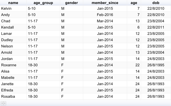
The initial step is to have sample data. Simply enter the data below into a new Google Sheets file in the range A1:F16 and name the tab “Master,” or use the provided button to copy the sample sheet.

Sample Sheet

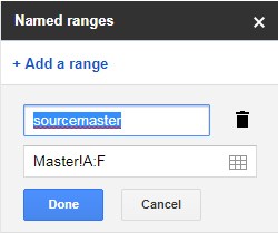
You should name this range (not required if you use my sample sheet as I have already named it) to simplify the formula. Naming ranges is the most effective way to improve the readability of a formula.

To achieve this, navigate to the Data menu and select Named Ranges. Assign the range name “sourcemaster” as shown below.

Note: You can now utilize LET to name ranges directly within the formula itself.

Filter Text Field

You can observe various age groups listed under the “age_group” field. I am utilizing the QUERY function to filter the “age_group” field for the group “11-17” in a new sheet in the same Google Sheets file/Workbook.

Formula:

=QUERY(sourcemaster, "select A, B, C, D, E, F where B='11-17' ", 1)

In the above query formula, “sourcemaster” is the named range you just created in the “Master” sheet, and A, B, C, D, E, and F are the columns that you want to extract.

The QUERY function syntax is as follows:

QUERY(data, query, [headers])

As mentioned earlier, you can use the QUERY function as an alternative to the FILTER function in Google Sheets. Here is the equivalent FILTER formula:

=FILTER(sourcemaster, CHOOSECOLS(sourcemaster, 2)="11-17")

If you analyze the outputs, you can see that the QUERY retains the header, whereas the FILTER doesn’t.

If you wish to learn more about the FILTER function, refer to our tutorial on filtering data into separate sheets in Google Sheets.

Filter Date Field

In the previous Google Sheets QUERY formula, we applied a text field as the criterion, namely “11-17”. When utilizing a date as a criterion in QUERY, follow the formula below.

=QUERY(sourcemaster, "select A, C where F = date '1999-09-20'", 1)

I employed the QUERY function to filter the “dob” (date of birth) field in the data on the sheet “Master”. The resulting output will include only the names and genders.

Here is the alternative FILTER function:

=FILTER(CHOOSECOLS(sourcemaster, {1, 3}), CHOOSECOLS(sourcemaster, 6)=DATE(1999, 9, 20))

Refer to the following two tutorials to gain a comprehensive understanding of correctly using the date as a criterion in the QUERY function:

1. Convert Date to String Using the Long-winded Approach in Google Sheets
2. How to Use Date Criteria in Query Function in Google Sheets

Filter Numeric Field

If you wish to use a number as a criterion in QUERY, follow the example below.

Using the same sample data as above, let’s apply the function to filter the data based on the “age” field.

=QUERY(sourcemaster, "select A, B, C, D, E, F where E = 24", 1)

This formula filters the “age” field where the age of members is 24.

Here is the equivalent FILTER formula:

=FILTER(sourcemaster, CHOOSECOLS(sourcemaster, 5)=24)

Conclusion

In all the examples above, we specified the criterion within the formula. However, you can use a cell reference instead. To learn more about using cell references in Google Sheets QUERY, refer to: “How to Use Cell Reference in Google Sheets Query.”

I hope you have gained an understanding of how to use the QUERY function as an alternative to the FILTER function in Google Sheets.

The provided examples are straightforward, especially if you create the sample dataset first and apply the formulas on your own.

For a more in-depth understanding of this function, please refer to the tutorials below:

1. How to Use Month Function in Google Sheets Query
2. Filter by Month and Year in Query in Google Sheets
3. How to Use the Datediff Function in Google Sheets Query
4. How to Use LIKE String Operator in Google Sheets Query
5. CONTAINS Substring Match in Google Sheets Query for Partial Match
6. How to Use Not Equal to in Query in Google Sheets
7. How to Use Arithmetic Operators in Query in Google Sheets
8. How to Sum, Avg, Count, Max, and Min in Google Sheets Query
9. How to Use Query with Importrange in Google Sheets
10. STARTS WITH and NOT STARTS WITH Prefix Match in Google Sheets Query
11. Ends With and Not Ends With Suffix Match in Query
12. How to Use And, Or, and Not in Google Sheets Query
13. Simple Comparison Operators in Google Sheets Query
14. How to Use Multiple OR in Google Sheets Query
15. How to Use DateTime in Query in Google Sheets
16. Examples of the Use of Literals in Query in Google Sheets
17. Multiple CONTAINS in WHERE Clause in Google Sheets Query
18. How to Offset Match Using Query in Google Sheets