How to Use Cell Reference in Google Sheets QUERY

Using cell references in the ‘query’ performed in the Google Sheets QUERY function can be a little tricky because it’s treated as a string. For example, consider the following formula:

=QUERY(A1:C, "SELECT *", 1)

In this formula, A1:C represents the ‘data’, “SELECT *” is the ‘query’, which is a string, and 1 represents the ‘headers’ as per the syntax QUERY(data, query, [headers]).

In Google Sheets, the QUERY function uses a WHERE clause to filter data based on conditions you specify. This clause helps you extract only the rows that match your criteria.

You can hardcode the criteria within the ‘query’ or enter them in cells and refer to those cells in the formula. In this tutorial, I’ll detail the latter, which involves specifying cell references in the ‘query’ part of the QUERY function.

When referencing a cell that contains a condition, in most cases, we need to use at least one of the simple comparison operators or complex string comparison operators such as MATCHES and CONTAINS.

Using Cell References in Google Sheets QUERY with Simple Comparison Operators

In this section, let’s learn how to use cell references in Google Sheets QUERY when utilizing the simple comparison operators listed below.

Equal to: =
Not equal to: != or <>
Greater than: >
Less than: <
Greater than or equal to: >=
Less than or equal to: <=

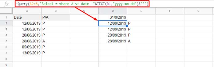
In my sample data, column A contains dates, and column B contains text values (‘P’ for present and ‘A’ for absent).

Let’s say the date criterion is stored in cell D1, which is ’31/08/2019′ in the DD/MM/YYYY format (if your Sheets’ default date format is MM/DD/YYYY, enter the criterion in that format in cell D1). You can reference cell D1 within the WHERE clause as follows:

=QUERY(A2:B, "SELECT * WHERE  A<= DATE '"&TEXT(D1, "yyyy-mm-dd")&"' ", 0)

Note: I’ve used the range A2:B to exclude headers.

Query Where Clause Criterion as Cell Reference

The above expression is a date literal (literals are values such as strings, numbers, Boolean TRUE/FALSE, or different date/time types used for comparisons or assignments).

If the criterion is a string and you want to refer to the cell containing the criterion, for instance, cell F1, use it as ='"&F1&"'

For example, to filter A1:B where column B is equal to “P”, then use the QUERY formula as follows:

=QUERY(A1:B, "SELECT * WHERE B ='"&F1&"' ", 0)

The given sample data doesn’t include a numeric field. Let’s assume you have data in columns C and D and want the QUERY to return column C if D is equal to 100.

Enter the criterion 100 in cell E1.

=QUERY(C2:D, "SELECT C WHERE D="&E1&" ", 0)

Similarly, you can use other comparison operators. Need more examples? Please check out this tutorial: Examples of the Use of Literals in Query in Google Sheets

That concludes the usage of cell references in QUERY with simple comparison operators.

Using Cell References in Google Sheets QUERY with Complex Comparison Operators

The purpose of using complex comparison operators is for string/substring comparison in the QUERY function.

In various tutorials, I have explained the use of complex comparison operators such as Contains, Matches, Like, Starts With, and Ends With for string/substring matching. However, in those tutorials, instructions on how to use cell references in the WHERE clause were not included. Let’s explore those usages below.

When Using ‘Contains’:

I have sample data in column A. I want to filter the data that contains a specific word entered in cell C1.

See the formula used in cell C2 below to understand how I have used the cell reference C1 as the criterion along with the Contains operator in the ‘query’ string.

=QUERY(A2:A, "SELECT A WHERE A CONTAINS '"&C1&"' ",0)

Criterion from a Cell in CONTAINS Sheets in Query

When Using ‘Matches’:

Among all string comparison operators in Google Sheets QUERY, Matches, which is a (preg) regular expression match, is somewhat complex. So, you may refer to my dedicated tutorial to learn its usage. Here we will see two examples to understand using cell references in this context.

The Matches substring match in the formula below takes the criterion (regular expression) from cell C1.

=QUERY(A2:A, "SELECT A WHERE A MATCHES '"&C1&"' ", 0)

Matches Operator Criterion from a Cell in Query

The regular expression is .*Project 1|.*Project 2, which matches all the strings ending with either Project 1 or Project 2.

When Using ‘Like’:

Let’s explore how to use a cell reference as a criterion in the Like Operator (for wildcard match) within Google Sheets QUERY function.

Example #1: % (Percentage) Wildcard as Cell Reference

=QUERY(A2:A, "SELECT A WHERE A LIKE '"&C1&"' ",0)

In the following illustration, pay special attention to the criterion used in cell C1, which is %Project 1. The Percentage wildcard in QUERY is similar to the asterisk wildcard (matches zero or more characters of any kind) used in other native Google Sheets functions.

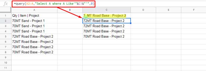
Sheets Query Like Operator with Criteria from a Cell

Example #2: _ (Underscore) Wildcard as Cell Reference

In this case, the cell reference in the ‘query’ string remains the same as the above example. Thus, no changes are required in the formula, except for the criterion in cell C1, which is 7_MT Road Base - Project 2. The underscore wildcard is used to match any one character similar to the question mark wildcard used in other native Google Sheets functions.

Query Like Operator Underscore Wildcard Reference from a Cell

When Using ‘Starts With’ and ‘Ends With’:

By now, you should have a good understanding of the QUERY syntax for using a cell reference within it.

Let’s see how to use a cell reference in the Query Starts With and Ends With operators.

Query Cell Reference – ‘Starts With’ Syntax:

Type “70MT” in cell C1 and use the below formula to return the strings in column A that start with the substring “70MT”:

=QUERY(A2:A, "SELECT A WHERE A STARTS WITH '"&C1&"' ",0)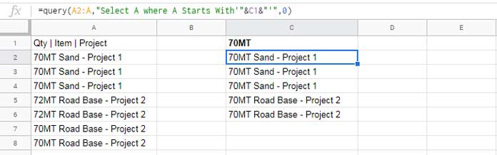

Starts With Criterion as Cell Reference in Query

Query Cell Reference – ‘Ends With’ Syntax:

The Query ‘Ends With’ cell reference syntax is almost the same as the Query ‘Starts With’.

=QUERY(A2:A, "SELECT A WHERE A ENDS WITH '"&C1&"' ",0)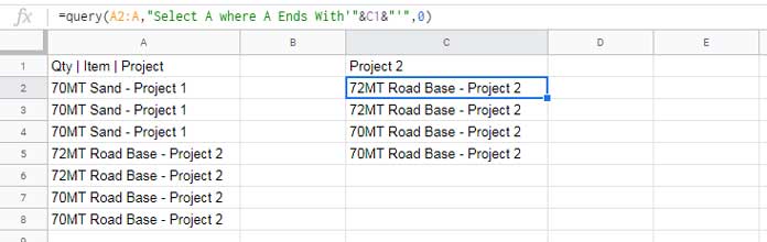

Ends With Criterion as Cell Reference in Query

Before using this formula, enter the criterion “Project 2” in cell C1 to return all the values in column A that end with the substring “Project 2”.

Conclusion

In all the above examples, you can make the formulas case-insensitive by wrapping column identifiers, such as A, and cell references, such as C1, with the LOWER function.

Example:

=QUERY(A2:A,"SELECT A WHERE LOWER(A) MATCHES '"&LOWER(C1)&"'",0)

That’s all. Enjoy!

27 COMMENTS

Daniel September 28, 2023 At 5:34 pm

Hi Prashanth,

I need to change the column number every day from Col10 to Col11, where Col'"&CEL VALUE&"'. Can you help please?

- Prashanth September 29, 2023 At 12:58 pm
  
  Hi Daniel,
  
  Please check out this tutorial: Google Sheets QUERY: Select Different Columns Each Day
  
Guy August 23, 2023 At 11:02 pm

Hi Prasanth,

First of all, thank you for sharing this site with us, and I’d like to express my deep respect for its quality and teaching methods.

I would need your expertise on the following subject.

=QUERY(IMPORTRANGE("Sheet_ID", "sheet1!B2:o"), "Select Col3,Col1,Col10,Col14,Col5 where upper(Col14)='"&upper(L1)&"'")

The QUERY only returns the results that match the data manually entered and never the data that matches the calculated data.

Hoping to have been clear.

Could you give me an indication of my problem?

Regards

- Prashanth August 24, 2023 At 9:37 am
  
  Hi Guy,
  
  Thanks for your kudos!
  
  I understand that the values in column 14 are text strings from the criterion usage in the QUERY function.
  
  Here are some troubleshooting tips:
  
  1. Check the formula in column 14. It may return white spaces.
  2. Replace upper(Col14) = '"&upper(L1)&"' with upper(Col14) contains '"&upper(L1)&"'
  
  I hope this helps!
  
karimulla June 12, 2023 At 5:30 pm

Hi Prasanth,

Here is my Query formula.

=QUERY(Master!$A:$R,"Select J where L='"&Final Dash!L2&"' Limit 10",1)

Can you help me with this? Where am I going wrong?

- Prashanth June 13, 2023 At 10:53 am
  
  Hi, karimulla,
  
  You were very close. Please check this.
  
  =QUERY(Master!A:R,"Select J where L='"&'Final Dash'!L2&"' Limit 10",1)
  
  When the sheet name contains space, use an apostrophe on both sides of the name.
  
Anand Gaur January 26, 2023 At 1:52 pm

=QUERY(A2:B,"Select * where B = "&J2&" ")

Where J2 is number 15000. No Error, but no answer.

- Prashanth January 27, 2023 At 11:26 am
  
  Hi, Anand Gaur,
  
  Make sure that column B doesn’t contain text values.
  
Vijay Sihamr December 26, 2022 At 12:15 am

=QUERY('Sheet1'!A1:Z,"select Sum(Count(R),Count(S),Count(T), Count(U)) where B Matches '"&AH4:AH&"' and '"&AI4:AI&"' IN(R,S,T,U)",0)

Can anyone help me?

- Prashanth December 27, 2022 At 2:41 pm
  
  Hi, Vijay Sihamr,
  
  You can find the correct way to use the following syntax in my tutorial Multiple CONTAINS in WHERE Clause in Google Sheets Query.
  
  where B Matches '"&AH4:AH&"'
  
  What do you mean by IN(R,S,T,U)?
  
Haris November 26, 2022 At 11:47 pm

Hello,

I need to get output if one of the C5 or C6 is empty.

=QUERY(Sheet1!A1:G30, "select * where D='"&C5&"' and C='"&C6&"' ")

Any help is greatly appreciated! Thank you!

- Prashanth November 27, 2022 At 9:20 am
  
  Hi, Haris,
  
  Please use WHERE 1=1 in the SELECT clause that will help you use multiple IF statements within the Query formula.
  
  =QUERY(Sheet1!A1:G30, "select * where 1=1 "&if(C5="",,"and D='"&C5&"'")&if(C6="",,"and C='"&C6&"'"))
  
Cate November 24, 2022 At 2:54 pm

How do I use a cell reference for the first argument (range) in the query function, please?

I have a query related to drawing data from several daily report sheets 01.11, 02.11, 03.11, etc.

So the query formula works if I input the ranges manually for data from rows where there were sales.

=query ({'04.11'!A3:W100;'05.11'!A3:W100;'06.11'!A3:W100}, "select * where Col5>1",1)

Looking forward to your advice – Thank you.

- Prashanth November 25, 2022 At 10:47 am
  
  Hi, Cate,
  
  That’s doable now using my REF_SHEET_TABS named function!
  
  Please check my tutorial “Reference a List of Tab Names in Query in Google Sheets” for more info.
  
Barry Phelps February 17, 2022 At 4:06 am

I need to select specific columns based on user input.

So I need to have the query perform SELECT A, B, C if a user chooses those columns, or it could be E, G, Y if a user selects different columns.

Is it possible to have "select '"&$B$4&"' where…?

- Prashanth February 18, 2022 At 10:10 am
  
  Hi, Barry Phelps,
  
  It’s possible. But not as above.
  
  E.g.:-
  
  =query(A5:Z,"Select "&B4&" where B is not null")
  
  You can insert single or multiple column IDs in B4.
  
  Single Column: A
  Multiple Columns: A, X, Z
  
Xabiso February 14, 2022 At 1:30 pm

Hi, thanks for this helpful insight. If I want to reference one column, how could I possibly go about this?

- Prashanth February 18, 2022 At 9:28 am
  
  Hi, Xabiso,
  
  This may help – How to Use Multiple OR in Google Sheets Query.
  
Frank February 4, 2022 At 10:24 pm

Hi, again Prashanth,

I’m using the Query function frequently, but now I have problems with a query that exceeds the Z column. My code looks like this;

=query(Answers!$A1:$Z200, "select A,B,X where A ...")

When I change $Z200 to $AH200, it shows the result of A1, B1, and so on in the correspondent column of the first line, nothing more.

Any idea?

- Prashanth February 5, 2022 At 9:54 am
  
  Hi, Frank,
  
  Specify the header in the formula as below.
  
  E.g.:-
  
  =query(Answers!$A1:$Z200, "select A,B,X where A is not null",1)
  
  If that doesn’t help, if possible, share your sheet URL via “Reply” below. I won’t publish it.
  
Sunil Thakur May 31, 2021 At 10:16 pm

In this line in this article;

=query(A2:A,"Select A where A Matches '"&C1&"'",0)

There is an extra double quote at the end of ‘”&C1&”‘”

Thanks for the article.

- Prashanth June 1, 2021 At 7:54 am
  
  Hi, Sunil Thakur,
  
  The SELECT clause starts with opening double-quotes. That last one is to close that.
  
  This may help?
  
  QUERY(data, "Select......", [headers])
  
David Sarnowski June 1, 2020 At 10:41 pm

First of all, thank you! I appreciate this article very much.

I am using Google Query with an importrange function so I have to use Col# to reference things. My query works perfectly and if I type in the " order by Col2 asc" the query sorts as expected.

If I write the query to look like "order by '"&B2&"' asc" and cell B2 contains "Col38", the query does not sort.

I have a dropdown feeding cell B2 so I can ideal dynamically sort my query. Any thoughts on why this is not working?

- Prashanth June 2, 2020 At 1:56 pm
  
  The same I’ve already noted in the 4th paragraph of this tutorial starting with “As a side note…”. If you read from that paragraph you will get the link to the relevant tutorial.
  
  Still, to save your precious time, I am providing the solution in the form of an example formula. Please pay your attention to the Select clause.
  
  =query({A1:E4},"Select * order by "&F2&" asc")
  
  The difference here is the “column identifier” as a cell reference, not a criterion/condition.
  
  I hope this makes sense.
  
  Cheers!
  
Nana April 17, 2020 At 12:44 pm

Hello, this is my formula:

=QUERY(AB6:AW,"Select AB, AC, AD, AE, AF, AG, AH, AI,AJ,AK,AL,AM,AN,AO,AP,AQ,AR,AS,AT,AU,AV,AW where AI >= '"&AC4&"'",0)

…and it gives input of N/A.

AI is a column of sizes in Numbers where AC4 is the minimum value of the sizes.

Can you help me out?

- Prashanth April 17, 2020 At 12:54 pm
  
  Hi, Nana,
  
  Change '"&AC4&"'",0) to "&AC4&"",0)
  
  If you want to master the use of ‘Literals’ use in Query, I have already one post. Search “Literals” within this post to find the relevant link.
  
  - Nana April 20, 2020 At 7:32 am
    
    Thank you so much, Prashanth!