This tutorial explains how to specify multiple CONTAINS for partial matching strings in the WHERE clause in Google Sheets Query.

Besides aggregation, the QUERY function in Google Sheets showcases excellent capabilities for string matching. This feature significantly enhances the tool’s ability to perform advanced data filtering.

There are simple comparison operators and five complex string comparison operators to achieve that. The complex string comparison operators are CONTAINS, MATCHES, LIKE, STARTS WITH, and ENDS WITH.

Some of you may already be well aware of the use of CONTAINS and its counterpart, NOT CONTAINS, in Query. Here is an example:

Example 1 (Formula in cell D1): Extract all the ‘Product Codes’ that contain the string ‘ABC’.

=QUERY(A1:A, "SELECT * WHERE A CONTAINS 'ABC' ", 1) // case-sensitive
=QUERY(A1:A, "SELECT * WHERE LOWER(A) CONTAINS 'abc' ", 1) // case-insensitive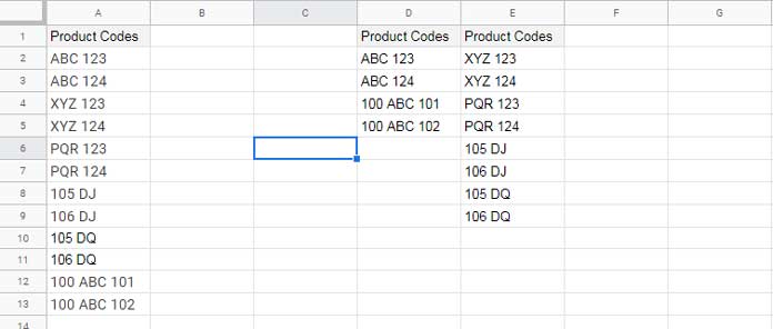

Example 2 (Formula in cell E1): Extract all the ‘Product Codes’ that do not contain ‘ABC’.

=QUERY(A1:A, "SELECT * WHERE NOT A CONTAINS 'ABC' ",1) // case-sensitive
=QUERY(A1:A, "SELECT * WHERE NOT LOWER(A) CONTAINS 'abc' ", 1) // case-insensitive

The purpose of using multiple CONTAINS in the Query WHERE clause is to perform multiple substring matches. Let me address that issue, which is the main topic of this post.

Note: You can enter the string to match in a cell, for example, in cell F2, and refer to that cell as follows: '"&F2&"'. This means you should replace 'ABC' (or 'abc') with '"&F2&"' in the above formulas.

Multiple CONTAINS in the QUERY Function and Practicality Issues

Of course, we can use multiple CONTAINS in the QUERY function WHERE clause for multiple substring matches. First, let’s see how to do that.

We can use the following QUERY formula to filter column A where the rows partially match ‘ABC’ or ‘XYZ’ (case-sensitive):

=QUERY(A1:A, "SELECT * WHERE A CONTAINS 'ABC' or A CONTAINS 'XYZ'", 1)

This works wonderfully. However, the issue arises when the number of strings to match increases, requiring many ‘CONTAINS’ and OR logical operators to separate each CONTAINS. This makes the formula longer and more difficult to manage.

So, how do we properly use multiple CONTAINS in the QUERY function WHERE clause?

Let’s find out.

MATCHES: The Alternative to Multiple CONTAINS in Query

Before we proceed with multiple substring matches, let’s replace our D1 and E1 formulas first. We will replace CONTAINS in those formulas with MATCHES.

MATCHES in WHERE Clause (Example Formula in cell D1):

=QUERY(A1:A, "SELECT * WHERE A MATCHES '.*ABC.*' ",1)

NOT MATCHES in WHERE Clause (Example Formula in cell E1):

=QUERY(A1:A,"SELECT * WHERE NOT A MATCHES '.*ABC.*' ",1)

When replacing CONTAINS with MATCHES, ensure to include .* around the criterion. If you want to refer to a cell, for example, cell F2, where you have entered ABC, replace '.*ABC.*' with '.*"&F2&".*'.

Examples of Multiple Partial Matches of Strings

In the earlier examples, I extracted the ‘Product Codes’ that contain/don’t contain the substring ‘ABC’. Now I am going to demonstrate multiple substring matches/mismatches in Query formulas.

See the following formulas:

Formula in D1:

=QUERY(A1:A,"SELECT * WHERE A MATCHES '.*ABC.*|.*DJ.*' ", 1)

Formula in E1:

=QUERY(A1:A, "SELECT * WHERE NOT A MATCHES '.*ABC.*|.*DJ.*' ", 1)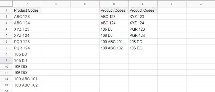

When replacing a single criterion CONTAINS with multiple criteria MATCHES, in addition to the .* around the criterion, include a | separator between the strings. This allows us to include several partial matching as well as non-matching criteria in a single Query.

Yes! MATCHES-based string matching is my answer to how to use multiple CONTAINS in the WHERE clause in Google Sheets Query.

Specifying a Criteria Range in MATCHES in Query

Assume the conditions (substrings) to match are entered in B2:B3, where ABC is in B2 and DJ is in B3. Then you can replace '.*ABC.*|.*DJ.*' (regular expression) in the formula with the following code:

ArrayFormula("'"&TEXTJOIN(".*|", TRUE, ".*"&TOCOL(B2:B3, 1))&".*'")

Just replacing that regular expression won’t suffice. Use the formula as follows:

=QUERY(A1:A,"SELECT * WHERE A MATCHES "&ArrayFormula("'"&TEXTJOIN(".*|", TRUE, ".*"&TOCOL(B2:B3, 1))&".*'")&" ", 1)

In the above code, the TOCOL function ensures that blank cells, if any, in the criteria range are removed, and the TEXTJOIN function joins the values placing a .*| delimiter in between.

This is the dynamic way to use multiple CONTAINS in the WHERE clause in Google Sheets Query using MATCHES substring match.

Before concluding, here’s one bonus tip. Do you know how to use CONTAINS and NOT CONTAINS in a single Query?

CONTAINS and NOT CONTAINS in a Single Query Formula

Here, for two criteria partial match, one containing and the other not containing, you can use CONTAINS in the WHERE clause. For single as well as multiple conditions (matches/mismatches), use MATCHES.

Single Condition CONTAINS and NOT CONTAINS:

=QUERY(A1:A, "SELECT * WHERE A CONTAINS 'ABC' AND NOT A CONTAINS 101", 1)

Multiple MATCHES and NOT MATCHES (Multiple CONTAINS and NOT CONTAINS):

=QUERY(A1:A, "SELECT * WHERE A MATCHES '.*AB.*|.*DJ.*' AND NOT A MATCHES '.*101.*|.*102.*' ", 1)

Resources

• How to Aggregate Strings Using Query in Google Sheets
• How to Offset Match Using Query in Google Sheets
• MATCH Function in Query WHERE Clause in Google Sheets