I don’t have seen anybody performing Offset Match using Query so far in Google Sheets. So I hope this is a fresh content for you!

I know the title is a little clumsy. I have tried to make it shorter without losing the meaning but without success, right?

What do you mean by Offset Match using Query?

It simply means offset a certain number of rows based on a matching keyword.

Using Google Sheets Query, you can Offset a given number of rows using the Offset clause.

If you put “Offset 5” the Query formula would offset 5 rows. Here the number 5 is the so-called ‘given number of rows’.

You can replace this offset number with a Match function based formula. What is the benefit of doing so?

In a one dimensional array, you can use a search key in the Match formula to return the relative position of that key in that array/range. Then use that number to offset in Query.

Offset Match Using Query in Google Sheets – Example

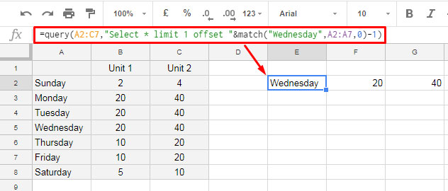
Here is one example.

This tutorial is actually about the use of Match function in Query formula Offset clause.

The above Query formula finds the search key “Wednesday” in column A and offset up to that row.

Actually, the above Query formula is an Index Match alternative! Index Match is an all-time popular spreadsheet combination formula for lookup and offset.

The Match matches a value and Index uses that match value to offset. That is called Index Match and that is what I have done with the Query formula above.

Can you show me the Index Match formula then?

Here you go!

=index(A2:C,Match("Wednesday",A2:A,0))

Now I am going to show you how the above same result I am replicating with the Match in Query.

I have already a very detailed tutorial on the Index Math. So I am not going to that detail.

I am going to elaborate on the Query formula that I have used in the example screenshot above that has lots of potential in data manipulation.

Offset Match Using Query – Formula and Explanation

Formula:

=query(A2:C,"Select * limit 1 offset "&match("Wednesday",A2:A,0)-1)

In both the formulas, I mean the Index Match and Query Match, I have used the same Match formula.

For your quick reference here is the Syntax of Match in Google Sheets:

MATCH(search_key, range, [search_type])

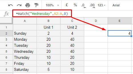
The search key used in Match is “Wednesday” and its relative position in the given dataset is 4.

In Index, you can use this 4 (Match formula) as it is (please scroll back and see the formula). It returns the 4th-row values.

But in Query, you should only offset 3. If you set offset number to 4, the formula would offset 4 rows and will return the value from the 5th-row.

So I have used the Match formula in Query as below.

match("Wednesday",A2:A,0)-1

See the minus 1 at the end.

So the Query formula is equal to;

=query(A2:C,"Select * limit 1 offset 3")

You have learned a new trick in Google Sheets that is how to Offset Match Using Query.

What is the benefit of the Offset Query over Index Match?

Index Match vs. Offset Match Using Query – Key Benefits

The Query is more flexible. You can play around with the Limit clause in Query to return a certain number of rows after Match offset.

Example Formula 1:

=query(A2:C,"Select * limit 2 offset "&match("Wednesday",A2:A,0)-1)

Result:

Example Formula 2:

=query(A2:C,"Select * offset "&match("Wednesday",A2:A,0)-1)

In this formula, I have excluded the limit clause. So the formula would offset the first 3 rows and returns the rest of the rows as it is.

That means Offset Match Using Query in Google Sheets has a certain edge over Index Match in terms of data manipulation.