Purpose of WHERE 1 Equals 1 in Google Sheets QUERY

If you’ve worked with SQL or Google Sheets Query, you may have seen something unusual:

WHERE 1=1

At first glance, it looks pointless—1=1 is always true. So why use it?

In this post, I’ll explain the purpose of WHERE 1=1 in Google Sheets Query and show you a practical example where it makes your formulas simpler and more flexible.

This tutorial is part of the WHERE Clause in Google Sheets QUERY: Logical Conditions Explained hub, which covers all logical operators, comparisons, and condition-building patterns used in QUERY statements.

Table of Contents

Why Use WHERE 1=1?

The WHERE clause filters rows based on conditions. For example:

=QUERY(A1:A,"SELECT A WHERE A = 'Apple'")

returns only rows with “Apple.”

Note: The QUERY function is case-sensitive, so Apple is different from apple. To make it case-insensitive, you can use upper() or lower() in your query, e.g., =QUERY(A1:A, "SELECT A WHERE upper(A) = 'APPLE'").

But sometimes, you want:

All rows if a cell says All Fruits
Filtered rows if a cell says Apple, Orange, etc.

Google Sheets QUERY updating to show all rows when 'All Fruits' is selected

This is where WHERE 1=1 comes in handy. It acts as a dummy first condition that’s always true, so you can safely attach extra conditions with AND later.

Example Dataset for Dynamic QUERY

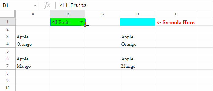
Let’s say column A contains fruit names. Cell B1 has a drop-down with values:

All Fruits
Apple
Orange

Step 1: Return All Rows

Both formulas below return the same result (all rows):

=QUERY(A1:A,"SELECT A")
=QUERY(A1:A,"SELECT A WHERE 1=1")

So WHERE 1=1 doesn’t change the result—it just sets up the formula for flexibility.

Step 2: Add a Dynamic Condition

Dynamic Filter Based on Drop-Down

Now let’s make the filter depend on B1.

=QUERY(A1:A,"SELECT A WHERE 1=1 "&IF(B1="All Fruits",""," AND A = '"&B1&"'"))

Formula Breakdown

WHERE 1=1 acts as a placeholder first condition.
IF(B1="All Fruits", "", ... ) decides whether to add a second condition.
AND A = '"&B1&"' adds the filter when a specific fruit is selected.

Handling “All Fruits” Selection

If B1 = All Fruits → =QUERY(A1:A,"SELECT A WHERE 1=1") → returns all rows.

Handling Specific Fruit Selection

If B1 = Apple → =QUERY(A1:A,"SELECT A WHERE 1=1 AND A = 'Apple'") → returns only “Apple.”

Header Argument in QUERY

Note: In the above examples, we omitted the header argument, so QUERY will automatically choose 1 (data has a header) or 0 (data has no header). To explicitly specify a header, use:

=QUERY(A1:A,"SELECT A WHERE 1=1 "&IF(B1="All Fruits",""," AND A = '"&B1&"'"), 1)

Here, 1 indicates the first row is a header.

Why Not Skip WHERE 1=1?

Without WHERE 1=1, you’d have to write a more complex formula with IF inside the query string. Using WHERE 1=1 makes it easier to append multiple conditions dynamically with AND, OR, etc.

Key Takeaways

WHERE 1=1 always evaluates to true.
It’s a trick to simplify formulas when adding optional conditions.
Great for drop-down filters (e.g., “All” vs. specific value).
Remember, QUERY is case-sensitive by default; use upper() or lower() to make it case-insensitive.