How to Use the Datediff Function in Google Sheets Query

DATEDIFF is one of the scalar functions in Google Sheets Query, which returns one value per row. It doesn’t aggregate the data.

There are three types of functions and operators for data manipulations in Google Sheets Query: Aggregation functions, Scalar functions, and arithmetic operators.

The above comes in the first category.

To learn the DATEDIF worksheet function, please follow the date functions guide.

The DATEDIFF function in Query (see the double “F”) returns the date difference between two dates or timestamp values.

On the other hand, the DATEDIF is far more advanced and can return the number of days, months, years, etc., between two dates.

DATEDIFF Function in Google Sheets Query: Example

First, you can learn how to find the difference between two dates using the DATEDIFF scalar function in Google Sheets Query.

Then you can experiment with some real-life examples like;

How to find the upcoming birthdays using Query?
How do we extract the expiring contracts within one month, 30 days, or any specific number of days?

1. Find the Number of Days Between Two Dates in the Query

Syntax:

dateDiff(end date, start date)

We can use this Query scalar function in a date or DateTime column.

The formula will return integer values because it truncates time values before calculation.

Sample Data:

I have a few work start dates in column A and work end dates in column B.

Let’s see how to use the DATEDIFF function in Google Sheets Query to return the number of days between the given work start and end dates in each row.

Formula (D1):

=QUERY(A1:B,"Select A,B,dateDiff(B,A)")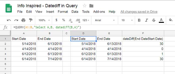

The datediff function in Query - example

You can just use =QUERY(A1:B,"Select dateDiff(B,A)") to return one column with the number of days.

DATEDIFF in Query Vs DATEDIF Worksheet Function: Differences

The DATEDIF is a stand-alone worksheet function, whereas the DATEDIFF is a scalar function for use inside Query.

DATEDIF is feature rich. We will only consider how the formulas differ in returning the difference in days between two date or DateTime values.

If I use the worksheet function in cell D1, the formula must be like this.

It’s like;

=ArrayFormula(datedif(A2:A5,B2:B5,"D"))

It’s as per the following syntax where the “D” represents days.

datedif(start date,end date,unit)

Regarding the difference with DATEDIFF, here, the start date comes first in the order.

The above difference is related to syntax, but the following one is related to calculation.

If we accidentally specify a start date greater than the end date, the scalar function will return a negative number, whereas the worksheet one will return the #NUM error.

Real-life Use of the DATEDIFF Function in Google Sheets Query

Please go through the below two examples.

1. Finding the Upcoming Birthdays Using a Query Formula

Here my sample data is like this.

Column A contains the date of birth of a few persons. Their names are in column B.

=ArrayFormula(QUERY({A2:B,{(date(year(today()),month(A2:A),day(A2:A)))}},"select Col1,Col2 where Col2<>'' and dateDiff(Col3,now())=30"))

I’ve used the above Query formula in cell D2.

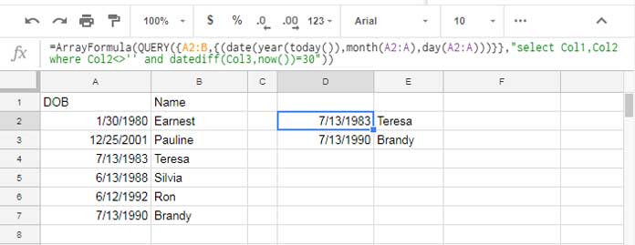
It returns the DOBs and names whose birthdays are coming in 30 days from today’s date.

Formula Explanation

In this example, there are two columns: DOB (A) and Name (B).

We have virtually added a third column that extracts the months and days from column A and adds the current year to form a date.

For example, the DOB of the person in cell A2 is 1/30/1980.

With the below formula, we can change only the year part of this date.

=date(year(today()),month(A2),day(A2))

I’ve used the DATEDIFF function inside the Query formula to find the number of days between today’s date with this newly formed date.

datediff(Col3,now())

If the result is 30, Query selects those DOBs and Names, else it returns an #N/A error.

2. Extracting the Expiring Contracts Within One Month, 30 Days, or N Days

If you could understand the above example, solving this problem is easy.

Here is how to use the DATEDIFF function inside the Query for that.

=QUERY({A2:B},"select Col1,Col2 where Col2<>'' and dateDiff(Col1,now())=30")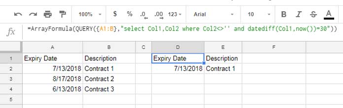

extract the rows containing expiry dates

You can change the =30 to >30 or any other number to set a different expiry.

Additional Tips

Above, I have used the NOW() function to return today’s date. It’s hardcoded inside the formula.

If it’s in a cell, e.g., in cell C1, use the below formula.

=QUERY({A2:B},"select Col1,Col2 where Col2<>'' and dateDiff(Col1,date '"&TEXT(C1,"yyyy-mm-dd")&"')=30")

That’s all about the use of the DATEDIFF function in Google Sheets Query.

13 COMMENTS

John January 28, 2022 At 1:11 pm

This is more of a general question relating to DATEDIF.

I am calculating years, months, and days using the DATEDIF formula based on the total number of days.

Here is the formula with total days being in cell A1.

=DATEDIF(0,A1,"y")&" years – "&DATEDIF(0,A1,"ym")&" months – "&DATEDIF(0,A1,"md")&" days"

My question: Months in the DATEDIF formula are considered full or complete months. Does this mean in my case where there are only days to calculate and no start date or end date, that complete months would mean the average number of days in a calendar month which is something like 30.437.days?

I’ve looked all over the web to find an answer and can’t see one.

- Prashanth January 31, 2022 At 10:25 am
  
  Hi, John,
  
  Please analyze the below formulas (both are equal).
  
  Formula 1:
  
  =datedif(0,64,"D")
  
  Formula 2:
  
  =datedif(date(1899,12,30),date(1899,12,30)+64,"D")
  
  Try replacing “D” with “MD” in both the formulas. I hope that clarifies.
  
Ted Stapenhorst October 14, 2020 At 8:46 am

Hi Prashanth,

I have 4 columns:

Location | Tested | DateOfTest | EmployeeType
District Office | Yes | 10/01/2020 | Staff
Maintenance | Yes | 10/10/2020 | Staff

I took your Query, modified it, and put it in F2 or the E column is blank:

=ArrayFormula(QUERY({A2:D,{(DATE(YEAR(TODAY()),MONTH(TODAY()),DAY(TODAY())))}},"SELECT Col1,Col3,Col4 WHERE Col4 is not null AND datediff(Col3,Col5)<=14"))

I'm trying to pull out the rows where Col3 <= 14 days from today. I'm getting a REF error. Any help would be appreciated.

- Prashanth October 16, 2020 At 12:22 pm
  
  Hi, Ted Stapenhorst,
  
  Try this Query;
  
  =ArrayFormula(QUERY({A2:D},"SELECT Col1,Col3,Col4 WHERE Col4 is not null and Col3<=date '"&TEXT(today()-14,"yyyy-mm-dd")&"'"))
  
  or the following Filter.
  
  =filter({A2:A,C2:D},C2:C<=today()-14)
  
Nessus October 3, 2019 At 12:04 pm

Great… thank you very much.

So, it’s not possible to add also a text value to the formatted cells?

- Prashanth October 3, 2019 At 12:51 pm
  
  Only two values like the text “Ended” in the highlighted cells and the text “Pending” in the cells which are blank (not highlighted).
  
  On my shared example Sheet, I have used the following formula in cell C3.
  
  =ArrayFormula(if($C$1:$AG$1>=AH3,"Ended",))
  
  which then copied to C5 and C7.
  
  - Nessus October 3, 2019 At 1:20 pm
    
    Yes, but what if there are data before the ENDED date cell ?… then the ArrayFormula will not expand.
    
    - Prashanth October 3, 2019 At 2:00 pm
      
      Array formula requires blank cells to work. If not, it will return the #REF error. That’s why I omitted the array formula in my first reply.
      
      - Nessus October 3, 2019 At 2:45 pm
        
        So there is no other way to do this?… some script maybe?
        
        On another issue. If the expiry date it’s not yet set, then show empty cells.
Nessus October 2, 2019 At 10:44 pm

Ok… this is my sample file…

– File copied and link removed by Admin –

I’ve edited one row manually to show you what I am trying to do.

Thanks

Nessus

- Prashanth October 3, 2019 At 11:21 am
  
  Hi, Nessus,
  
  On your Sheet, I have applied the required conditional formatting rule.
  
  Here is a copy of your Sheet. In this copy, the range to highlight is C3:AG7 based on the dates in row#1 and column AH.
  
  https://docs.google.com/spreadsheets/d/1ry_ZXw02dAEiDDTy6alhHO4ZO4fbQM-WVPpVe8fbcQY/copy
  
  Formula Rule: =and(C$1>=$AH3,datevalue($AH3)>=1)
  
  The locale of this Sheet is UK. Since your Sheets’ locale is Greece, there the ' in the formula is replaced by a ;.
  
  Best,
  
Nessus October 2, 2019 At 3:11 pm

Hello there,

I have a question about this.

I have a sheet in sort of calendar format but the dates are as headers in one row on the top, the dates of the week are below in another row and the data are entered in the third-row below.

Now, I want to highlight/format the cells in the row containing the data based on the date that will be specified in a separate cell that is in the same row at the end of it.

Basically it’s a planner.

Thanks

Nessus

- Prashanth October 2, 2019 At 8:25 pm
  
  Hi, Nessus,
  
  Please show me a demo Sheet.
  
  Best,