QUERY dates by month name means filtering a date column by the month’s name (like “January” or “June”) instead of using the month number in Google Sheets.
This approach is especially helpful when you’re working with drop-downs containing month names from January to December, rather than month numbers from 1 to 12. Just a quick note: when you query dates using month numbers, Google Sheets treats months as 0 to 11 — where 0 is January and 11 is December — not 1 to 12.
One of the key advantages of querying dates by month name is its clarity for users. A month name in a dropdown is generally more readable and user-friendly than a number.
This tutorial is part of the Date Logic in QUERY hub.
Learn how date logic works in Google Sheets QUERY, including date criteria, month-based filtering, and DateTime handling.
How to QUERY Dates by Month Name in Google Sheets?
To QUERY dates by month name in Google Sheets, we first need to convert the month name criterion into a month number. For example, if you want to filter by “June”, you can use:
=MONTH("June"&1)This will return the month number 6.
Why does that work?
When you write "June"&1, it becomes "June1", which Google Sheets interprets as a date like June 1 of the current year (e.g., 01/06/2025). The MONTH function then extracts the number 6 from that date. We only care about the month here, not the year.
Using It in QUERY
Now let’s look at how to use this in a QUERY formula to filter dates by month name.
Example: QUERY Dates by Month Name in Google Sheets
Assume:
- Column A contains sales dates.
- Column B contains sales quantities.
You want to filter for all transactions that occurred in January.
Using Month Number:
=QUERY(A1:B, "Select * where month(A)+1=1", 1)Why month(A)+1?
Because the MONTH function in QUERY returns months as 0 (Jan) to 11 (Dec), so we add 1 to make it more intuitive (1 to 12).
QUERY by Month Name:
Start by isolating the month number like this:
=QUERY(A1:B, "Select * where month(A)+1="&1, 1)Now, replace the number 1 with a formula that converts a month name to a number. For example, using “January”:
=QUERY(A1:B, "Select * where month(A)+1="&MONTH("January"&1), 1)That’s how you filter a date column by month name in a QUERY formula in Google Sheets.
What if the Month Name Is in a Cell?
In most practical cases, you’ll be using a dropdown or cell reference for the month name. Suppose you have a dropdown in cell D1 with month names from January to December. You can plug that into the formula like this:
=QUERY(A1:B, "Select * where month(A)+1="&MONTH(D1&1), 1)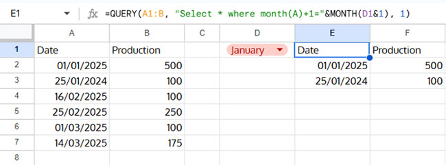
Filter Date Column by Month Name and Year
If your data spans multiple years, you might want to filter by both month name and year.
For example, to filter for January 2025:
=QUERY(A1:B, "Select * where month(A)+1="&MONTH("January"&1)&" and year(A)=2025", 1)If the month name is in D1 and the year is in D2, the formula would be:
=QUERY(A1:B, "Select * where month(A)+1="&MONTH(D1&1)&" and year(A)="&D2, 1)FAQs
Can I Use Abbreviated Month Names?
Yes, you can! The formula works the same way. Just make sure to use standard three-letter abbreviations like Jan, Feb, Mar, etc.
Does the December Month Issue Affect This?
Nope! An empty cell returns month number 12 by default, but since we’re not modifying the original date values directly, the formula won’t mistakenly include empty rows.


