This post explains how to use date values in Google Sheets Query. Date value means the date in number format, which is a recognizable date.
For example, the date value of 03/11/2020 (3rd November 2020) in Google Sheets will be 44138. You can test it in the following ways.
- Enter the said date in any cell and format that cell to a number from the menu Format > Number > Number.
- By using the formula =DATEVALUE(“03/11/2020”) (the dates within double quotation marks will be as per the format dd/mm/yyyy or mm/dd/yyyy depending on your Sheets’ settings).
Sometimes we may have a date value column in our data because of the following.
- Imported Data.
- Formula output.
Since I don’t have such data to explain how to use the date value in Google Sheets Query, I am converting dates to numbers.
As a side note, this post is not about how to use date criteria in Query.
Introduction
To manipulate a date column, we can use the Query as below.
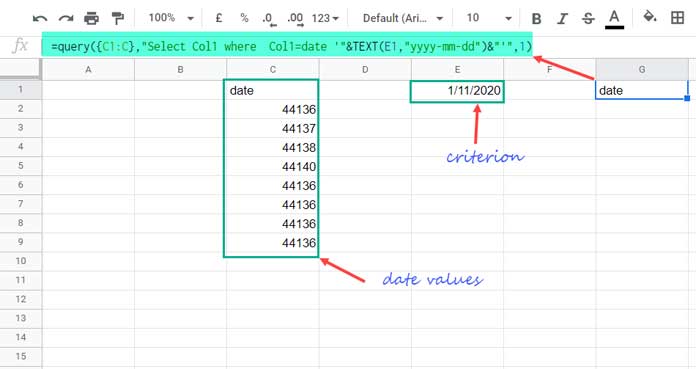
=query({C1:C},"Select Col1 where Col1=date '"&TEXT(E1,"yyyy-mm-dd")&"'",1)This formula filters all the dates in C1:C, which matches the date in E1, i.e., 01/11/2020.
Now let’s format the dates in C1:C manually to date serial numbers.
Select C2:C, then go to the Format menu > Number > Number.
Now you can see that the Query formula in G1 returns only the header, no other values.

Let’s see how to use date values in Google Sheets Query after one more example of the problem.
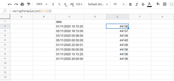
This time I am using the INT function in a DateTime column.
Let’s understand what happens when we use INT in the timestamp/DateTime column.

I have used INT to extract the dates from the timestamp. The result will be date serial numbers.
Now time to learn how to use the date values in Google Sheets Query.
1. Imported Data Contains Date Values and Its Use in Query
Suppose our imported data has a date serial number column. How do we use the Query formula in such a date value column?
We have two options to choose from and here are them.
- Using Number Literal in the Criteria.
- Using the Format Menu to Format the Date Values.
Let’s start with the simplest one.
Option # 1: Number Literal Instead of Date Literal in the Criteria Part
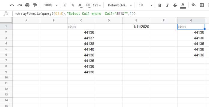
Assume the data in C2:C is imported or manually converted to date serial numbers.
The following Query formula in cell G1 filters those date values using the date condition in cell E1.
=ArrayFormula(query({C1:C},"Select Col1 where Col1="&E1&"",1))
In the above Query formula, I have used number literal (Col1="&E1&") instead of the date literal (Col1=date '"&TEXT(E1,"yyyy-mm-dd")&"') in the criteria part.
Related: Examples of the Use of Literals in Query in Google Sheets.
The output of the formula will also be in number format. Just include to_date to format it to dates.
=ArrayFormula(TO_DATE(query({C1:C},"Select Col1 where Col1="&E1&"",1)))Option # 2: Using the Format Menu
If you format the imported data in C2:C back to date from the Format menu, then you can use the Query as usual with the date literal in the condition part.
=query({C1:C},"Select Col1 where Col1=date '"&TEXT(E1,"yyyy-mm-dd")&"'",1)2. Data Contain Date Values Due to a Formula (Expression as Query Data)
Here is one more example of how to use the date values (date serial numbers) in Google Sheets Query.
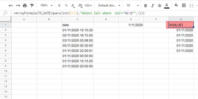
Here the INT converts the date to date values. So we can’t use the Format menu here as there is no physical column with date serial numbers to format.
If we use the numeric literals in Query, the formula will be as follows.
=ArrayFormula(query(int(C1:C),"Select Col1 where Col1="&E1&"",1))We can optionally include the To_date as earlier.
=ArrayFormula(TO_DATE(query(int(C1:C),"Select Col1 where Col1="&E1&"",1)))
The error value in the first row of the result is due to the INT trying to convert the header row in the data, which is a string, to date.
Using the Label clause, we can easily remove that error (replace the error value with the required header).
=ArrayFormula(TO_DATE(query(int(C1:C),"Select Col1 where Col1="&E1&" label Col1'date'",1)))If we use date literal, we should move the To_date to inside Query (wrap INT instead of Query).
=ArrayFormula(query(to_date(int(C1:C)),"Select Col1 where Col1=date '"&text(E1,"yyyy-mm-dd")&"' label Col1'date'",1))That’s all about how to use date values (date serial numbers) in Google Sheets Query.
Thanks for the stay. Enjoy!


Dear Prashanth,
I tried your revised codes, and I’m amazed. It works 🙂
You are so kind, and your patience with all the queries here is so long.
I hope you never stop helping me and others.
Again and again, thank you so much for your help.
Good job.
Dear Sir/Madam,
I have a problem with my sheet.
Scenario:
I have a timestamp (column 1) with the employee name (column 2) in sheet 1.
In sheet 2, I use your query codes to transfer all the data from sheet 1 to sheet 2 with the date today only.
=QUERY(EmployeesResponse!A1:B,"Select * where B is not null and A contains date '"&text(E7,"yyyy-mm-dd")&"'")The problem is that every 1st of the month, all the dates with the number “1” are mixed in this day.
Example: May 1, 2022
Other dates mixing: May 10, 11, 12, 13, 14, 15, 16, 17, 18 and 19.
I hope you can help me with my problem.
I appreciate your prompt response to my query 🙂
Thank you in advance.
Hi, Jay-ar,
Try to avoid using the Contains operator with Query as it’s for string/text comparison.
You can use the todate scalar function instead as below.
=QUERY(EmployeesResponse!A1:B,"Select * where B is not null and toDate(A)=date '"&text(E7,"yyyy-mm-dd")&"'")