When working with grouped data in Google Sheets, filtering becomes problematic if the group labels aren’t repeated in each row. In such cases, Google Sheets treats the blank cells as distinct entries, which makes it difficult to apply filters or run functions like QUERY or SUMIF.
A quick and dynamic solution is to use a helper column that repeats the group labels. This guide shows you how to do that using an array formula, so your data becomes filter-friendly without manual duplication.
What Are Group Labels in Google Sheets?
Group labels are the category names used to organize your data, usually found in the first column. Subgroup labels may appear in subsequent columns. If these labels are only shown once at the top of each group and left blank in the following rows, filtering won’t work correctly.
Example Problem
In the table below:
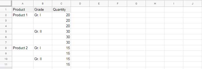
Filtering this table for Product 1 returns only the first row, because the rest have blank group labels in column A.
Why Repeat Group Labels?
By repeating group and subgroup labels in every row, Google Sheets can correctly filter and aggregate grouped data. This approach is especially helpful when using:
- Filters
- QUERY
- SUMIF or SUMIFS
- Pivot tables
How to Repeat Group Labels Using a Helper Column
Let’s use a helper column (e.g., column E) to repeat the group labels in column A.
Step 1: Repeat Group Labels
Paste this formula in cell E1:
=ArrayFormula(
   VSTACK(
      "Helper1",
      IF(
         ROW(A2:A) <= MATCH(2, 1/(C:C<>""), 1),
         LOOKUP(ROW(A2:A), ROW(A2:A)/(A2:A<>""), A2:A),
         ""
      )
   )
)
This formula fills down the group labels in column A into column E.
Step 2: Repeat Subgroup Labels
To do the same for subgroups in column B, paste this formula in cell F1:
=ArrayFormula(
VSTACK(
"Helper2",
IF(
ROW(B2:B) <= MATCH(2, 1/(C:C<>""), 1),
LOOKUP(ROW(B2:B), ROW(B2:B)/(B2:B<>""), B2:B),
""
)
)
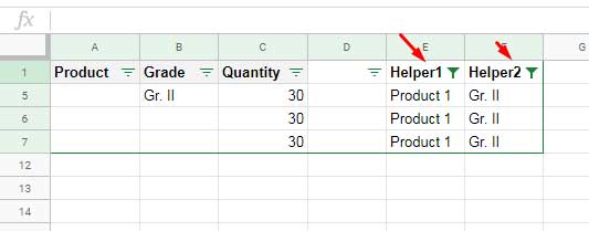
)Now columns E and F contain repeated group and subgroup labels.
How These Formulas Work
Let’s break down the formula in E1:
ROW(A2:A): Creates an array of row numbers starting from row 2.A2:A<>"": Checks where column A is not blank.LOOKUP(...): Fills blank cells by copying down the last seen non-blank value.MATCH(2, 1/(C:C<>""), 1): Finds the last non-empty row in column C to limit the formula’s range.VSTACK("Helper1", ...): Adds a column header for the helper column.
How to Filter Using the Helper Columns
After adding the helper columns:
- Select columns A–F.
- Go to Data > Create a filter.
- Use the dropdown in column E (Helper1) to filter by group (e.g., “Product 1”).
- Use the dropdown in column F (Helper2) to filter by subgroup if needed.
This ensures all relevant rows are included in your filtered result.
What If My Group Labels Are in a Different Column?
If your group labels aren’t in column A, just update the formula accordingly:
- Replace
A2:Awith the actual column (e.g.,D2:D). - Ensure
ROW(...)aligns with the range starting from your data’s second row. - Adjust the
MATCH(...)part if your data ends based on a different column.
Conclusion
If your grouped data is missing repeated labels, Google Sheets won’t filter correctly. Using a helper column with the right array formula lets you repeat group labels dynamically, enabling accurate filtering and easier analysis.
Related Tutorials
If you’re interested in similar techniques used in this tutorial, check out these posts:
- Fill Blank Cells with the Next Non-Empty Value in Google Sheets – An alternative method that fills each blank with the next value below it.
- Fill Blank Cells with Values from the Cell Above in Google Sheets – Learn how to automatically carry forward the last non-empty cell using a dynamic formula.
- Find the Address of the Last Used Cell in Google Sheets – Learn how to locate the last non-empty cell in a column, even if the data has blanks.


