Google Sheets doesn’t offer a built-in menu command to fill blank cells with values from the cell above in a column. To accomplish this, you need to use a formula in Google Sheets.
Using a non-array formula, it’s straightforward to fill blank cells in a column with the value from the cell just above. However, there is also an Array Formula that can achieve this.
Let me first show you the non-array formula, which will provide a foundation for understanding the Array Formula later in this tutorial.
Here’s the formula used in cell C2, copied down the column:
=IF(LEN(B2), B2, C1)
Regardless of the data type, this formula will copy the value from the cell above and fill the blank cells below.
For an array formula approach to fill blank cells with values from the non-blank cell above, we can use one of two methods:
- Using a lookup function.
- Using the SCAN LAMBDA function (a newer method).
We’ll start with the lookup function method, though the latter is simpler to implement.
Auto Fill Blank Cells with Values from Above in Google Sheets Using LOOKUP
Assume there are values in the range B2:B15 with some blank cells in between. To fill those blank cells with values from the cell above, use the following formula in cell C2:
=ArrayFormula(LOOKUP(
   ROW(B2:B15),
   ROW(B2:B15)/(B2:B15<>""),
   B2:B15
))
This is an array formula, so you do not need to copy-paste or drag the fill handle of C2 down.
Formula Explanation
The core function in the formula is LOOKUP, and here’s how it works to fill empty cells with values from the non-empty cell above:
Syntax:
=LOOKUP(search_key, search_range|search_result_array, [result_range])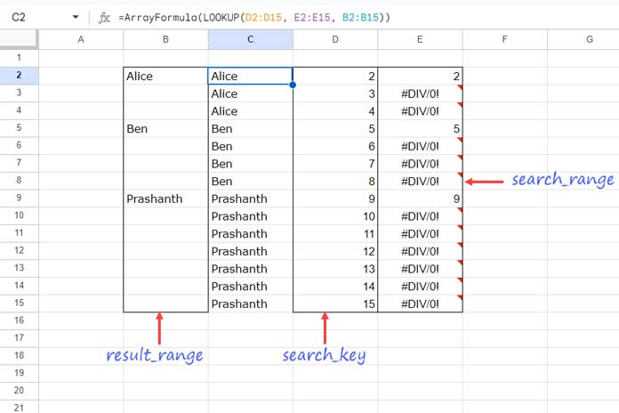
In the formula:
search_key:ROW(B2:B15)– This returns the row numbers for the data range when used with ArrayFormula.search_range:ROW(B2:B15)/(B2:B15<>"")– This returns row numbers corresponding to non-empty cells and generates errors for empty cells.- part 1:
ROW(B2:B15)– Returns row numbers. - part 2:
(B2:B15<>"")– Returns TRUE for non-empty cells and FALSE for empty cells.
- part 1:
result_range:B2:B15
Here’s how the formula fills blank cells with values from the cell above:
The formula searches for the search_key (row numbers) in the search_range. For matching rows, it returns the corresponding values from B2:B15. If the search_key is not found (i.e., in error rows), the function will match the row number that’s immediately smaller than the search_key. For example, if row #3 is not present in the search_range, the formula will match row #2.
Auto Fill Blank Cells with Values from Above in Google Sheets Using SCAN
The SCAN function is one of the LAMBDA helper functions (LHF) in Google Sheets, known for calculating a running total of a column in one go. We can also use it to fill blank cells between non-blank cells in a column.
Replace the LOOKUP formula with the following SCAN formula:
=SCAN(, B2:B15, LAMBDA(accu, val, IF(val="", accu, val)))How Does This Formula Work?
The SCAN function takes three arguments: initial_value, array_or_range, and lambda.
initial_valueis set to blank.array_or_rangeis B2:B15.
In the LAMBDA function, accu and val are used to pass values to the formula:
The formula IF(val="", accu, val) means that if the value in the current row is empty, return the accumulator value (the value from the cell above); otherwise, return the current row’s value.
This effectively fills the blank cells with the value from the cell above.


Thank you! Just saved me hours (after spending hours trying to figure this out)! Building something critical for my job and now I can look like the hero, not the zero.
Hi, Dan,
Thanks for your feedback.
I’ll update this post ASAP to include a simple formula using the new SCAN function.
Please check back after 1-2 days.
Thanks for this formula.
I have a question because after inputting this formula, my data stops at the last result range column that has data.
There are more rows below that which are empty.
Is there something I can tweak to fill the last few rows? TIA
Hi, Bryan,
I have given two formulas. One (under step # 3) is for infinite rows, and the other (the first formula from bottom to top) is for just up to the last non-blank row.
It seems you are using the latter one.
In that case, if the column in question (range in use) is B2:B, and you want the formula to return values up to row # 500, go to B500 and tap the spacebar.
That will expand the formula up to that row.
Your formula is great but, I try to apply it based on a column that has to be the same.
It skips empty values instead of always looking above.
I’ve created an example sheet here: — address removed by admin —
Please advise how this can be done? Thank you!
Hi, Eddy A,
The reference column (cell range) in the MATCH part of the formula is important.
I have used that formula part to find the cell address of the Last Non-Empty Cell Ignoring Blanks in a Column.
I have corrected the formula in your sheet.
How could this be done in the same column?
Hi, ramiro,
Select the result, right-click and copy.
Then right-click, paste special and apply paste value in the column you want.
Hello Prashanth,
It was a very good example/explanation!
I have just one question:
– What modification would you have to do in order to copy the last line instead of the first one?
To make it easier, I created one shared document on the link:
— LINK REMOVED BY ADMIN —
What I need is to obtain the row number associated with the first and last line of each title, but using array formulas on the first row.
Hi, Rafael,
I have inserted the below two formulas.
First Row:
=ArrayFormula(if(B5:B16<>"",row(B5:B16),))Last Row:
=ArrayFormula(IFNA(VLOOKUP(B5:B16,{lookup(row(B5:B16),if(len(B5:B16),row(B5:B16)),B5:B16),ROW(G5:G16)},2,1)))I know you could read the first formula. Regarding the second formula, I would try to write a detailed tutorial soon. In the meantime, you can read my below tutorial to understand some of the logic used.
How to Use Sumif in Merged Cells in Google Sheets.
Thank you for sharing this mind-blowing formula. However, I wonder if there is any way to fill the value for a certain number of times? For example, suppose I just want to fill the “test” values down the column for 14 times.
Hi, Trang,
Here is a similar post/tutorial.
How to Insert Duplicate Rows in Google Sheets.
Thanks a lot, this helped!
One small thing I noticed is that in the final formula, you could have just written;
It’s a bit cleaner that way. I tested it and it works.
Hi, Josh,
Thanks for your feedback!
Tonnes of useful information on here! Thank you, sir/madame.
Thank you so much!! Really appreciate the explanation as well. Amazing!