We can use Sumif in merged cells in Google Sheets. Let’s learn more about this type of conditional sum below.
Unlike database applications, we can merge cells in spreadsheets. The option for the same you can find under the Format menu in Google Docs Sheets.
When we merge cells in our spreadsheet, we must understand that it’s at the cost of losing the database ‘structure’ of our entered data.
The merging of cells may make a huge difference (negative impact) in our data manipulation.
In a merged range, we may find it difficult or unable to use database functions and other functions like Sumif, Filter, Query, etc.
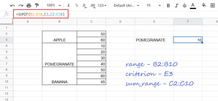
To make you understand the issue, let me use the below fruits’ data and a basic Sumif formula in cell F3.
=SUMIF(B2:B10,E3,C2:C10)
The Sumif formula in merged cells returns 10 instead of 100 (10+20+30+40) for the criterion “POMEGRANATE” (formula in cell F3 and criterion in cell E3).
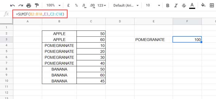
If you unmerge the cells and make the data similar to a database table, the formula would correctly return 100. See that example too.

But if you want to keep the merged cells and use the Sumif function, then you can find the correct formula below.
Sumif in Merged Cells in Google Sheets
When you merge a set of cells, for example, A1:A10, and type a value in this merged range, the value you entered will be recorded in cell A1, not in all the cells in the range A1:A10.
For example, select the range A1:A10 and click Format > Merge cells > Merge all. Then type “UK” in this merged range.
Type =A1 in any blank cell. The formula would return the value “UK”.
Change A1 with A2 in the formula and you can see that the formula now returns blank. That would be the case with other cells in this merged range.
That means, in this particular case, Sheets records the value “UK” only in cell A1, not in the range A1:A10.
So to use Sumif in merged cells in Google Sheets, we should replace the ‘range’ with a virtual range.
The role of the virtual range is to fill all the merged cells with values.
That means, as per our fruits’ data, fill B2:B3 with “APPLE”, B4:B7 with “POMEGRANATE”, and B8:B10 with “BANANA” (scroll up and see the very first screenshot).
Let’s code that formula first.
Virtual ‘Range’
Actually, for this, we can use different variations of a formula. Here I’m using the possibly simplest one.
First, I’ll use two helper column ranges that we can remove later on.
Helper Range 1
In cell H2, insert the below formula (let’s call it helper_formula_1) to return the row numbers of the cells that contain values in the range B2:B10.
=ArrayFormula(if(len(B2:B10),row(B2:B10)))The formula would return the following result.
| 2 |
| FALSE |
| 4 |
| FALSE |
| FALSE |
| FALSE |
| 8 |
| FALSE |
| FALSE |
From this what we can understand?
We can understand that B2 contains “APPLE”, B4 contains “POMEGRANATE”, and B8 contains “BANANA”. All the other cells in the range B2:B10 are blanks.
Now let’s go to the key step under “Helper Range 2” to perform the Sumif formula in merged cells in Google Sheets.
Helper Range 2
In cell I2, insert the below Lookup formula (let’s call it helper_formula_2).
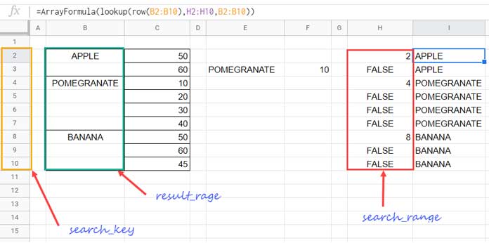
=ArrayFormula(lookup(row(B2:B10),H2:H10,B2:B10))The Lookup will populate the following result in I2:I10.
| APPLE |
| APPLE |
| POMEGRANATE |
| POMEGRANATE |
| POMEGRANATE |
| POMEGRANATE |
| BANANA |
| BANANA |
| BANANA |
It’s important to learn the above formula to understand how to Sumif in merged cells in Google Sheets.
To learn the above formula, first, refer to the Lookup syntax below that we have followed in the just above Lookup formula (as a side note, the Lookup function has two types of syntaxes).
Syntax: LOOKUP(search_key, search_range, result_range)
The search_key is the row numbers 2 to 10, the search_range is the helper_formula_1 result in H2:H10, and the result_range is B2:B10.

Lookup Rule: If the search_key is not found in the search_range, the item used in the Lookup will be the value that’s immediately smaller in the range provided. Didn’t get?
For example, the search_key 3 (row # 3) is not present in H2:H10. So Lookup will take 2 (immediately smaller in the search_range) as the search_key.
In the case of the search_keys 5, 6, and 7, the formula will consider it as 4. In the case of 9 and 10, the formula will consider it as 8.
So even if the search_key is the row numbers 2 to 10, the formula would read it as below.
| 2 |
| 2 |
| 4 |
| 4 |
| 4 |
| 4 |
| 8 |
| 8 |
| 8 |
So the corresponding values from B2:B10 will be returned.
Formula Example to Sumif in Merged Cells
We are almost set to use the Sumif in merged cells in Google Docs Sheets.
At the beginning of this post, I have given a Sumif formula (in cell F3) that returns a wrong result due to the merged cells. Here is that formula gain.
=SUMIF(B2:B10,E3,C2:C10)In this formula, we need to replace B2:B10 with the two helper formulas that we have written above.
Before replacing we need to first combine the two helper formulas which is pretty simple.
Just replace H2:H10 in the helper_formula_2 with the helper_formula_1 as below. That’s all that you want to do.
=ArrayFormula(lookup(row(B2:B10),if(len(B2:B10),row(B2:B10)),B2:B10))So we have combined the two helper formulas into one. Now we can use the combined formula to replace B2:B10 in the F3 formula as below.
=SUMIF(ArrayFormula(lookup(row(B2:B10),if(len(B2:B10),row(B2:B10)),B2:B10)),E3,C2:C10)
The above is an example to Sumif in merged cells in Google Sheets.
Resources:


The formula is terrific as I continue to inevitability deal with the team merging cells in the Google Sheets we share.
I’m having trouble with one thing and am not sure how to revise the formula to address it.
I have 24 columns, and I want a total of column I, which has dollar amounts based on the date in column T.
=SUMIF(ArrayFormula(lookup(row(T2:T4416),if(len(T2:T4416),row(T2:T4416)),T2:T4416)),B2,I2:I4416)
Cell B2 = 7/18/2022
Columns
Row # | Column I | Column T
3089 | $2,000 | 7/18/2022
3094 | $2,222 | (blank cell)
If I enter a “-” in the blank cell, it calculates the formula to only $2,000, which is the total I’m after.
Any suggestion on how to fix this is greatly appreciated!
Many thanks!
Hi, LeSha T.,
I assume you have merged cells in T2:T4416. Otherwise, you might have used a simple formula like this.
=sumif(T2:T4416,B2,I2:I4416)Now, to solve the issue, you must understand the reason.
In a vertically merged range, only the first cell contains the value. All other cells are blank.
My formula fills the blank cells in cell range T2:T4416 with the dates from just above cells.
While doing so, the formula fills all blank cells, whether within merged range or standalone.
So as you have suggested, leaving a hyphen in the cell that you want to skip will solve the issue.
But it’s not practical with several such cells. So do as follows.
1. Select T2:T4416.
2. Go to Format > Number > Plain Text (later, we will revert to date).
3. Go to Edit > Find and Replace.
4. In the “Find” field, input
^([\t]*)$and put a hyphen character in the “Replace with” field.5. Check “Match case” and “Search using regular expressions” and Done.
6. Then revert T2:T4416 to date.