Do you want to identify merged cells in a range? You can use formulas to find the addresses of merged cells in Google Sheets.
There are two approaches. One uses a formula combined with the Find & Replace command, whereas the second one uses a single formula, which is a lambda function.
I prefer the first approach if your data is very large, and the second one if it’s not so large.
The formulas will find and list all merged cell addresses. If A1:A5 is merged, the formula will return the child cell addresses, i.e., A2, A3, A4, and A5, not the parent A1. (There is no parent-child terminology. This is just for your understanding.)
If your purpose is just to unmerge all merged cells at once, you need to find the first merged cell in the range, and from that point select the range to unmerge and click Format > Merge Cells > Unmerge.
Option 1: List All Merged Cell Locations (Lambda Function)
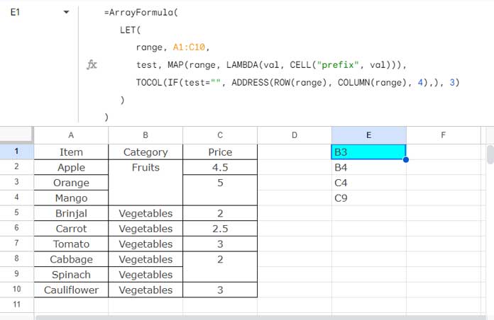
I have a sample dataset in A1:C10 where column A contains names of fruits or vegetables, column B contains categories, and column C contains prices.
Cells are merged in columns B and C. I want to find all child addresses of merged cells in the range A1:C10.
To do this, follow these steps:
- Select the range A1:C10.
- Click Format > Alignment > Center.
- Click Format > Number > Automatic.
- In cell E1, enter the following formula:
=ArrayFormula(
   LET(
      range, A1:C10,
      test, MAP(range, LAMBDA(val, CELL("prefix", val))),
      TOCOL(IF(test="", ADDRESS(ROW(range), COLUMN(range), 4),), 3)
   )
)
This formula will return the addresses of all merged cells in E1:E.
Formula Breakdown
(The formula breakdown is optional to read. You can skip it.)
Syntax: LET(name1, value_expression1, [name2, …], [value_expression2, …], formula_expression)
The purpose of the LET function is to ‘smoothen’ the formula, making it more reader-friendly and perform better. It simply assigns names to value expressions and uses those value expressions in the subsequent calculation(s).
- LET named the range A1:C10 with the name ‘range’.
- The value expression
MAP(range, LAMBDA(val, CELL("prefix", val)))is named ‘test’.
What does this ‘test’ do?
It’s a MAP lambda function that maps each value in the given array, the range A1:C10, to a new value by applying a lambda function.
The lambda function uses the CELL function, which returns the “prefix” of each cell. This prefix will be a “^” in all cells with values since we center-aligned the values in the range.
The formula expression TOCOL(IF(test="", ADDRESS(ROW(range), COLUMN(range), 4),), 3) returns the addresses of the cells whose values are empty in ‘test’. In this, TOCOL converts the result array into a list, removing empty cells.
That’s how it lists the child cell addresses of all merged cells in the range.
Option 2: List All Merged Cell Addresses (Find & Replace Support)
The above MAP lambda helper function may not be the best choice when you have data in hundreds of rows. If the above formula fails or slows down your Sheet, use this second approach.
Here, we will use a formula to list the cell addresses of all merged cells. Additionally, we will take support from the Find & Replace command in Sheets.
Here are the steps to follow:
Right-click on the tab name and click Duplicate (we will work on the duplicate sheet, not the original). In the duplicate sheet:
- Select A1:C10.
- Click Format > Number > Plain Text.
- Click Edit and select Find and Replace.
- In the Find field of the Find and Replace window, enter the
^([\t]*)$regex pattern. - In the Replace With field, enter
-. - Select “Search using regular expressions”.
- Make sure that Specific Range is selected against Search and the range is A1:C10.
- Click the Replace All button.
- Click the Done button.
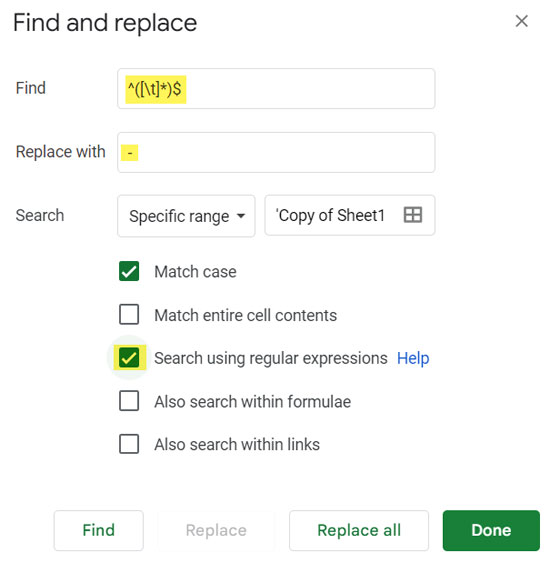
This will replace any blank cells in the range with “-“. You won’t see any difference if you use our sample data since there are no blank cells in the range.
Enter the following formula in cell E1:
=ArrayFormula(LET(range, A1:C10, TOCOL(IF(range="", ADDRESS(ROW(range), COLUMN(range), 4),), 3)))This formula will list the addresses of all merged cells (child, not parent) in E1:E. Actually, it returns the cell addresses of empty cells.
Wrap-up
We have seen two approaches to find the addresses of merged cells in Google Sheets.
Option 1 (Lambda Approach):
Requires you to center-align all the values in the range and then apply automatic formatting. The formula will take care of the rest.
It’s easy to use but may not be suitable if your data range is very large.
Option 2:
Here, we will work on a copy of the sheet since we want to modify the range using the Find & Replace command.
By replacing all blank cells with a hyphen or any other character using Find and Replace, the formula will take care of the rest.
This formula works better with large datasets.
Resources
- Find the Cell Address of a Last Used Cell in Google Sheets
- Address of the Last Non-Empty Cell Ignoring Blanks in a Column in Excel
- Array Formula to Convert Cell Addresses to Values in Google Sheets
- Get Cell Address of a Lookup Value in Google Sheets
- How to Fill Merged Cells Down or to the Right in Google Sheets
- Sequence Numbering in Merged Cells In Google Sheets


Thank you. Congratulations on finding merger cells. Kudos.