Automatically Fill Merged Cells in Google Sheets

Here, I’ll show you how to use an array formula-based approach to fill merged cells in Google Sheets, either down or to the right.

When you merge, say, ten cells in a column or row, only the first cell in the merged range actually holds a value. The rest are technically empty—even though visually it may seem like all the cells contain the same data.

That’s the problem.

By merging, you’re likely trying to convey that all those cells share the same value. While that works for presentation, worksheet functions don’t see it that way. So if you need to manipulate your data or use it in formulas, you’ll first need to fill merged cells in Google Sheets so each unmerged cell contains the correct value.

In this tutorial, I’ll show you how to do just that—vertically and horizontally.

Fill Merged Cells Down (Vertically) with Array Formula

Here’s a sample dataset:

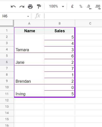
Sample data with merged cells in range A1:B11

Let’s say cells A2:A4 are merged with the value “Tamara,” A5:A6 are merged with “Jane,” and so on.

Here’s how to fill those merged cells with the correct values after unmerging:

Steps:

Note: Before unmerging, make sure to remove any empty rows that are not part of the merged cell ranges.

Select the range A2:A11 and unmerge the cells.
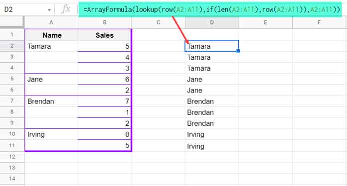
In cell D2, insert this formula:

=ArrayFormula(
   LOOKUP(
     ROW(A2:A11),
     IF(LEN(A2:A11), ROW(A2:A11)),
     A2:A11
   )
)

Array formula output filling merged cells down in Google Sheets

Select D2:D11, right-click, and choose Copy.
Click on cell A2, right-click, and choose Paste special > Values only.

That’s it! You’ve now filled the previously merged cells down using an array formula.

How Does This LOOKUP Formula Work?

Here’s the formula syntax explained:

LOOKUP(search_key, search_range, result_range)

search_key – Row numbers from 2 to 11.
search_range – Only rows that contain values in A2:A11 (others become FALSE).
result_range – The names from A2:A11.

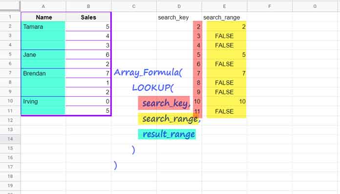
How LOOKUP fills down values in unmerged cells in Google Sheets

Google Sheets’ LOOKUP finds the last value less than or equal to the search key in the search range. So even if a direct match isn’t found, the last available value above it is used—perfect for filling down data.

Fill Merged Cells to the Right (Horizontally)

In the above example, we used ROW() for a vertical fill. To fill merged cells to the right in Google Sheets, we’ll use the COLUMN() function instead.

Sample Case:

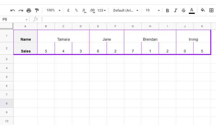
Suppose the cells in B1:K1 are merged.

Sample data with merged cells across columns in range A1:K2

Steps:

Unmerge B1:K1.
In cell B5, enter the following formula:

=ArrayFormula(
   LOOKUP(
     COLUMN(B1:K1),
     IF(LEN(B1:K1), COLUMN(B1:K1)),
     B1:K1
   )
)

Select B5:K5, copy it, and then paste values back into B1:K1.

That’s it—you’ve now filled merged cells to the right using an array formula.

Why This Method Helps

This method is especially helpful when dealing with large datasets. Instead of manually filling each merged cell, you can use this approach to automatically fill every unmerged cell with the appropriate value—either down or to the right.

If you’re working with large reports or dashboards, knowing how to fill merged cells in Google Sheets can save a lot of time and keep your data usable.

Final Tip

These formulas return dynamic results, meaning they’ll update automatically if you change the source data. If you want static values, copy the output and paste as values using Ctrl+Shift+V (or Cmd+Shift+V on Mac).