Google Sheets allows users to merge cells either horizontally or vertically. However, when it comes to sorting, you can’t directly sort vertically merged cells in Google Sheets.

That’s why I generally don’t recommend merging cells for formatting purposes—especially in datasets where sorting or filtering is needed.

I do occasionally use merged cells for layout or visual grouping, but never for data manipulation.

In short: if you plan to manipulate or analyze data, avoid merging cells in Google Sheets—or any other spreadsheet software.

That said, what if you’ve already merged cells vertically and now want to sort the data? Is there a workaround?

Yes! This post provides a practical solution to sort vertically merged cells in Google Sheets.

Example Table with Vertically Merged Cells

Let’s say we have the following data in range A1:B15, where some cells in column A are vertically merged:

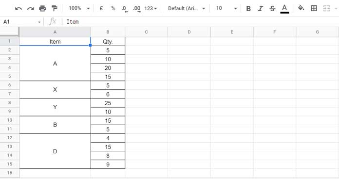
Here, the values “A”, “X”, “Y”, “B”, and “D” are merged across multiple rows in column A.

If you try to sort column A using Data > Sort range, you’ll get the notification: “You can’t sort a range containing vertical merges. There is a vertical merge at A2:A5.” If you instead try to use formulas for sorting, all the blank rows underneath the merged cells will be treated as empty, which causes sorting errors.

Understanding the Problem

Take the value “A” in cell A2. It appears merged over A2:A5, but only A2 contains the actual text; the rest (A3:A5) are technically blank. If you use =A2, it returns “A”, but =A3 or =A4 returns an empty string.

So when you attempt to sort a column with vertically merged cells, Google Sheets groups the blank cells together—separating them from their intended label. That’s the core issue.

Workaround: Sort Vertically Merged Cells in Google Sheets Using a Helper Formula

To fix this, we can fill the blank cells with the non-blank value above them using a formula, making sorting behave as expected.

Here’s the helper formula:

=ARRAYFORMULA(LOOKUP(ROW(A2:A15), ROW(A2:A15)/(A2:A15<>""), A2:A15))

This repeats each label down its corresponding rows, effectively “flattening” the vertically merged cells. You don’t need to enter this formula in the sheet—you’ll use it directly inside a sorting formula.

Learn more about this formula: Fill Blank Cells with Values from the Cell Above in Google Sheets

Option 1: Using the SORT Function

Let’s assume your data is in A2:B15.

You can use the HSTACK function to join the processed column A (with merged cells filled) with column B, then apply the SORT function.

Here’s the formula to sort vertically merged cells in Google Sheets using SORT:

=SORT(
   HSTACK(
      LOOKUP(ROW(A2:A15), ROW(A2:A15)/(A2:A15<>""), A2:A15), 
      B2:B15
   ), 1, TRUE
)

To sort in descending order, change TRUE to FALSE.

This will sort the data by the unmerged values in column A, maintaining the correct grouping of data.

Note: We don’t need to use ARRAYFORMULA within SORT.

Option 2: Using the QUERY Function

If you want more flexibility—like filtering out specific rows—you can use the QUERY function instead.

Here’s how to sort vertically merged cells using QUERY:

=QUERY(
   HSTACK(
      ARRAYFORMULA(LOOKUP(ROW(A2:A15), ROW(A2:A15)/(A2:A15<>""), A2:A15)), 
      B2:B15
   ), "SELECT * ORDER BY Col1 ASC"
)

To sort in descending order, change ASC to DESC:

... "SELECT * ORDER BY Col1 DESC"

To filter out specific items, say you want to exclude “A”:

=QUERY(
   HSTACK(
      ARRAYFORMULA(LOOKUP(ROW(A2:A15), ROW(A2:A15)/(A2:A15<>""), A2:A15)), 
      B2:B15
   ), "SELECT * WHERE Col1 <> 'A' ORDER BY Col1 ASC"
)

Note: QUERY is case-sensitive.

Conclusion

While there is no native way to sort vertically merged cells in Google Sheets, these formulas offer a solid workaround. Whether you use SORT for simplicity or QUERY for flexibility, both methods handle merged cells gracefully by simulating unmerged data.

For best practices:

• Avoid merging cells where sorting/filtering may be required
• Use helper formulas to simulate merged formatting if needed

Related Resources

• Copy-Paste Merged Cells Without Blank Rows/Spaces in Google Sheets
• Uncover Merged Cell Addresses in Google Sheets
• How to Use SUMIF in Merged Cells in Google Sheets
• How to Fill Merged Cells Down or to the Right in Google Sheets
• How to Use COUNTIF or COUNTIFS in Merged Cells in Google Sheets
• How to Use VLOOKUP in Merged Cells in Google Sheets
• Filtering When Columns Contain Merged Cells in Google Sheets
• XLOOKUP in Merged Cells in Google Sheets
• Creating Sequential Dates in Equally Merged Cells in Google Sheets
• Merge Duplicate Rows and Keep Latest Values in Excel