In Google Sheets, merging cells is not a good idea if you intend to manipulate your data. However, there might be reasons why you chose to merge cells in your dataset.

Suppose you need to look up a value using the XLOOKUP function in merged cells. How can this be achieved in Google Sheets?

To do this task, we will utilize a nested XLOOKUP formula. The inner XLOOKUP function will assist the outer XLOOKUP in searching for the key and returning the desired value.

Sample Data

The sample data is located in cells A1:C10. In this dataset, the first column contains employee names, the second column contains month names, and the third column contains their corresponding monthly salaries.

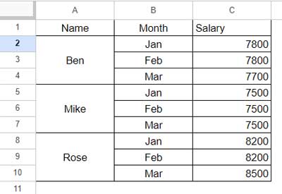
Please note that the employee names are merged cells. We will use an XLOOKUP formula to search for an employee’s name within this merged column and retrieve their salary (earliest or most recent) from the third column.

XLOOKUP Formula for Merged Cells

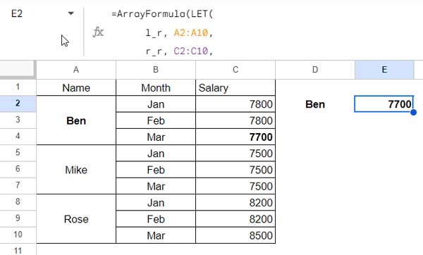
Cell D2 contains the employee name “Ben,” which serves as our search key.

The following XLOOKUP formula searches for the key in cell D2 within the merged cells in the first column and returns his most recent salary from the third column.

=ArrayFormula(LET(
      l_r, A2:A10, 
      r_r, C2:C10, 
      s_k, D2, 
      XLOOKUP(
          s_k, 
          XLOOKUP(ROW(l_r), IF(LEN(l_r), ROW(l_r)), l_r, ,-1), 
          r_r, ,0, -1
      )
))

The formula searches from bottom to top and returns the most recent salary. To achieve this, we’ve specified the search mode as -1 (highlighted in the formula).

If you want his earliest salary (search from top to bottom), use 1 as the search mode.

The formula follows the syntax:

XLOOKUP(search_key, lookup_range, result_range, [missing_value], [match_mode], [search_mode])

where:

• search_key: D2
• lookup_range: A2:A10
• result_range: C2:C10

You only need to specify these references and the highlighted search mode, and the formula will take care of the rest.

Now, you might be wondering how XLOOKUP can look up in the merged column and what workaround we have followed.

Formula Explanation

If you have vertically merged cells and enter a value in them, the value will appear in the topmost cell of the group. In our example, cells A2:A4, A5:A7, and A8:A10 are merged. Therefore, the employee names Ben, Mike, and Rose are located in cells A4, A5, and A8 only.

All other cells within the range A2:A10 are blank. Consequently, we need to fill the blank cells with the corresponding employee names. We will achieve this virtually, and that’s the logic behind XLOOKUP in merged cells.

In our formula, the following part accomplishes this task:

XLOOKUP(ROW(l_r), IF(LEN(l_r), ROW(l_r)), l_r, ,-1)

This part (inner XLOOKUP) acts as the lookup range in the outer XLOOKUP. But what does this formula do?

This XLOOKUP formula searches for the row numbers of the actual lookup range [ROW(l_r)] in the row numbers corresponding to employee names [IF(LEN(l_r), ROW(l_r))] and returns the corresponding employee names [ l_r ] in the matching rows.

The key aspect here is the match mode. It’s set to -1, which indicates an exact match or the next value that is lower than the search key. This effectively fills the column.

Please refer to the illustration:

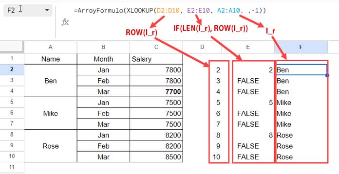
We utilize this resulting column as the lookup range in our outer XLOOKUP.

In summary, XLOOKUP itself is not capable of searching for keys in merged cells in Google Sheets. Therefore, we need to use another formula to generate a virtual array with values filled in merged cells. For this purpose, we have employed a second XLOOKUP.

Resources

• How to Use Sumif in Merged Cells in Google Sheets
• How to Use Sumproduct with Merged Cells In Google Sheets
• How To Use Countif or Countifs In Merged Cells In Google Sheets
• How to Use Vlookup in Merged Cells in Google Sheets
• How to Fill Merged Cells Down or to the Right in Google Sheets
• Array Formula to Fill Blank Cells With the Values from Cell Above