How to Use VLOOKUP in Merged Cells in Google Sheets (with Working Formulas)

Does VLOOKUP work with merged cells in Google Sheets?

Technically, yes. But it returns unexpected results if the lookup column contains merged cells. To fix this, you’ll need a formula that treats merged cells as if they were filled down.

In this tutorial, I’ll show how to use VLOOKUP with merged cells using two practical examples—so you always get the correct match, even from irregularly formatted tables.

Why VLOOKUP Fails with Merged Cells

When the lookup column has merged cells (like A1:A3 merged as “Mango”), VLOOKUP only matches the first row of the merged range. So =VLOOKUP("Mango", A1:C3, 3, 0) always returns the value from row 1—even if you want the price of Mango Grade 2 in row 3.

The Correct Way: Fill Down Merged Cells Virtually

To fix this, we’ll fill down merged cells virtually inside the formula, then combine that with other relevant columns before using VLOOKUP.

Example 1: Merged Item Column with Multiple Grades and Prices

Table:

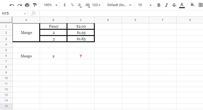
VLOOKUP with merged cells in Google Sheets – Mango price by grade example

Goal: Get the price of Mango, Grade 2.
Search values:

A6 = Mango
B6 = 2

Formula:

=ARRAYFORMULA(
   VLOOKUP(
      A6&B6, 
      HSTACK(LOOKUP(ROW(A1:A3), IF(LEN(A1:A3), ROW(A1:A3)), A1:A3)&B1:B3, C1:C3), 
      2, 
      FALSE
   )
)

How It Works:

LOOKUP(...) fills the merged cell values (like “Mango”) down to each row.
Combines Item & Grade to create a unique search key.
Then returns the corresponding value from the Price column.

Example 2: Lookup Structural Steel Weights from a Table with Merged Rows

Table in G8:I16:

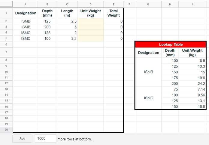
VLOOKUP with merged cells – structural steel weight lookup example in Google Sheets

Goal: From a sheet with:

A2:A = Type (e.g., ISMB, ISMC)
B2:B = Size (e.g., 125, 100)
…return the correct unit weight from the lookup table.

Formula (for cell D2):

=ARRAYFORMULA(
   VLOOKUP(
       A2&B2,
       HSTACK(LOOKUP(ROW($G$8:$G$16), IF(LEN($G$8:$G$16), ROW($G$8:$G$16)), $G$8:$G$16)&$H$8:$H$16, $I$8:$I$16),
       2,
       FALSE
   )
)

You can drag this down or convert it to a full array formula:

Full Column Array Formula:

=ARRAYFORMULA(
   IFNA(
      VLOOKUP(
         A2:A&B2:B,
         HSTACK(LOOKUP(ROW($G$8:$G$16), IF(LEN($G$8:$G$16), ROW($G$8:$G$16)), $G$8:$G$16)&$H$8:$H$16, $I$8:$I$16),
         2,
         FALSE
     )
   )
)

Key Takeaways

VLOOKUP fails in merged cells because it only reads the first row.
Use LOOKUP(ROW(), IF(LEN()), ROW(), range) to fill merged cells virtually.
Combine filled values with other columns to form a composite lookup key.
Wrap in ARRAYFORMULA to apply across multiple rows.