This tutorial describes two methods for merging values from two columns into one column in Google Sheets.
The first method combines values, such as merging first names from one column with last names from another. This is straightforward to do.
The second, less common method involves using a category column and another column. In this approach, the values from the second column are placed below each category. The values in the first column act as labels that separate the values in the second column.
Merge Values from Two Columns by Concatenating
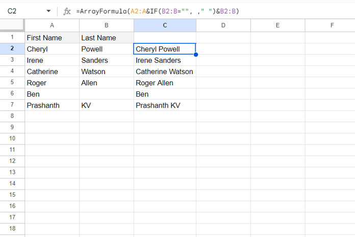
Assume you have first names in A2:A and last names in B2:B.
In cell C2, you can either enter the following formula and drag it down as far as needed:
=A2&" "&B2Alternatively, clear the contents of the range C2:C and enter the following array formula in cell C2:
=ArrayFormula(A2:A&" "&B2:B)These are the simplest ways to merge values from two columns into one column.
Sometimes, you might want to use a different character to separate values. In that case, you can replace " " with "-" to place a hyphen or use any other character you choose.
However, this approach may result in unwanted separators if the second column does not contain values. To handle this, you can use this formula:
=ArrayFormula(A2:A&IF(B2:B= "", "", "-")&B2:B)This formula removes the separator when the second column is empty. Similarly, if you are using a space as the separator, the formula would be:
=ArrayFormula(A2:A&IF(B2:B="", "", " ")&B2:B)This formula prevents adding a space character when no last name is present, even if it’s not visible.
The above methods are the simplest ways to merge values from two columns into one.
Merged List with Categories and Values in Google Sheets
This type of merging is useful when you have a category column and a value column to combine.
The sample data consists of weekday names in column A and sales values on those days in column B.
For instance, if three sales occurred on Monday, you will have “Monday” in three rows in one column and the corresponding sales values in another column.
After merging, the first row will contain “Monday,” followed by the three rows with the values from the second column. There will be multiple categories as well.
We can use two types of formulas to merge values from two columns this way in Google Sheets: with or without using LAMBDA functions.
Merge Values from Two Columns Without Using LAMBDA
The LAMBDA function is known to have performance issues when applied to very large datasets, so I would prefer this method. However, the LAMBDA approach has the advantage of being more flexible, which I will discuss later.
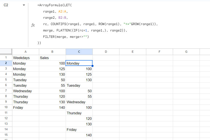
If your sample data is in A2:B and it’s sorted by column A, use this formula in cell C2 after clearing the contents in C2:C:
=ArrayFormula(LET(
   range1, A2:A,
   range2, B2:B,
   rc, COUNTIFS(range1, range1, ROW(range1), "<="&ROW(range1)),
   merge, FLATTEN({IF(rc=1, range1,), range2}),
   FILTER(merge, merge<>"")
))
Do you want to know how this formula merges values from A2:A and B2:B by using unique values in A2:A as row separators for B2:B?
Formula Explanation
The formula uses the LET function to assign names to the ranges A2:A and B2:B as range1 and range2, respectively.
COUNTIFS(range1, range1, ROW(range1), "<=" & ROW(range1)) calculates a running count of values in A2:A, where each category start is numbered 1. This running count is named rc.
FLATTEN({IF(rc = 1, range1,), range2}) – Here, the IF logical test returns values from range1 (A2:A) where rc (running count) equals 1. This is combined with the values from range2 (B2:B) using curly brackets. The FLATTEN function combines these two columns into a single column, named merge.
The issue with merge is that it may contain blank cells due to the flattening process.
FILTER(merge, merge <> "") removes these blank cells.
This generates a merged list with categories and values, where categories serve as separators.
Merge Values from Two Columns Using LAMBDA
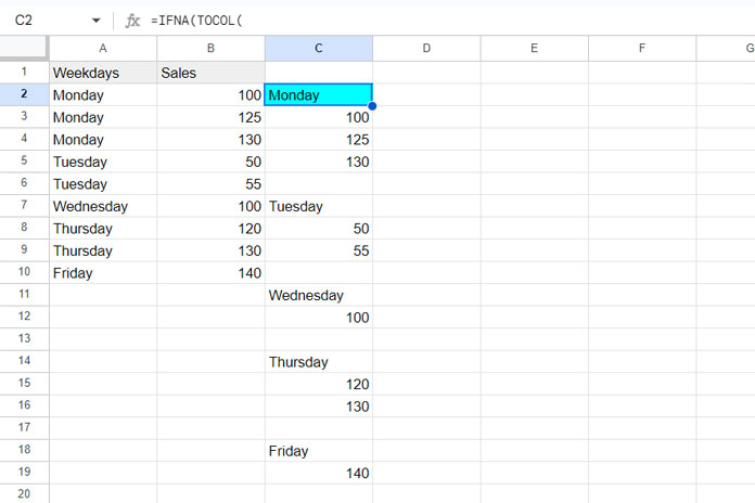
You can replace the previous formula with the following LAMBDA-based formula:
=IFNA(TOCOL(
   HSTACK(
        MAP(
           TOCOL(UNIQUE(A2:A), 1),
           LAMBDA(col, HSTACK(col, TOROW(FILTER(B2:B, A2:A=col))))
        )
   ), 1
))
This formula uses the MAP LAMBDA function to merge values from two columns.
Formula Breakdown
TOCOL(UNIQUE(A2:A), 1) returns unique categories and removes empty cells. The MAP function maps this array and applies the LAMBDA function to iterate through each value in the array.
| Monday |
| Tuesday |
| Wednesday |
| Thursday |
| Friday |
LAMBDA(col, HSTACK(col, TOROW(FILTER(B2:B, A2:A = col)))) – This LAMBDA function filters the values in B2:B based on the current value (col) from the array. TOROW transforms the output into a row. HSTACK appends the category value (col) with the filtered results.
| Monday | 100 | 125 | 130 |
The MAP function processes each value in the array, transforming the results into rows and appending them to the category value.
| Monday | 100 | 125 | 130 |
| Tuesday | 50 | 55 | |
| Wednesday | 100 | ||
| Thursday | 120 | 130 | |
| Friday | 140 |
TOCOL transforms the merged rows into a single column. The HSTACK function helps to insert empty rows between categories, and IFNA handles errors by replacing them with empty cells.
Adding Blank Rows Between Categories:
If you want to add blank rows below each category, you can specify " " within HSTACK, as shown below:
=IFNA(TOCOL(
   HSTACK(
        MAP(
           TOCOL(UNIQUE(A2:A), 1),
           LAMBDA(col, HSTACK(col, TOROW(FILTER(B2:B, A2:A=col))))
        ),""
   ), 1
))
This will leave one blank row below each category in the merged column. To add two blank rows, specify " ", " ".
Resources
- A Flexible Array Formula for Joining Columns in Google Sheets
- How to Remove Extra Delimiter in Google Sheets – Join Columns
- How to Left Join Two Tables in Google Sheets
- How to Right Join Two Tables in Google Sheets
- How to Inner Join Two Tables in Google Sheets
- How to Full Join Two Tables in Google Sheets
- Master Joins in Google Sheets (Left, Right, Inner, & Full) – Duplicate IDs Solved
- Anti-Join in Google Sheets: Find Unmatched Records Easily


Is there a way to put spaces between each day of the week?
Hi, Patrick,
See if this tutorial helps?
How to Automatically Insert a Blank Row below Each Group in Google Sheets.
Hi, Jordan!
Is it possible to apply the second method in Excel?
Hi Prashanth,
Is it possible to do the same as the above but insert the new group at intervals of 10 (assuming that there are always less than 8 values per day)?
i.e Monday and its values starting from C1, Tuesdays and it’s values starting from C11, Wednesday and it’s values starting from C21, etc.
So it won’t matter how many values are assigned to each day, the new group is started at the next interval.
Hi, Jordan,
I didn’t understand your question 🙁
Apologies, I have created an example sheet with a better explanation:
(URL has been removed by the Admin)
I’ve also added an extra request on the sheet to add a standard string between column A and column B when combining them.
Hi, Jodan,
Sorry! I don’t find a way to modify the current formula. But I do have some ideas. Here is it.
In the “New Example” tab, empty the columns D1:Z1.
Insert the below unstack formula in cell E1.
=ArrayFormula(transpose(trim(sort(split(transpose(query({transpose(unique((A2:A)));IF(len(B2:B),IF(transpose(
unique(A2:A))=A2:A,"-"&B2:B,""),"")},,1000)),"-")))))
The above formula is from my Unstack Data tutorial.
Then use the following Flatten in cell L1 to merge the two columns.
=flatten(transpose(F1:J10))Note: This is an untested formula. It has issues like sorting Weekdays in A-Z order.