Merging two tables in Google Sheets is a broad topic. Generally, it involves combining data from two separate tables into a single table. There are two main ways to achieve this:

Stacking Vertically: This method is used when both tables have similar column headers (e.g., months, weeks, categories). Stacking works even if the second table has fewer or more columns.

Joining Tables: This is a more controlled way to merge tables that share a common column (unique identifier). It is a broad topic that involves left, right, full, and inner joins. You should also know how to handle duplicate unique identifiers (IDs).

In this tutorial, we’ll focus on stacking vertically and a basic approach using a lookup formula to merge (join) tables based on a unique identifier.

For detailed tutorials on various join types and advanced merging techniques, check out the ‘Resources’ section below.

Merging Two Tables by Vertical Stacking in Google Sheets

In this example, the first table in A1:C4 contains three columns: Month, Sales Person, and Sales Volume, while the second table in E1:H5 contains four columns: Month, Sales Person, Location, and Sales Volume.

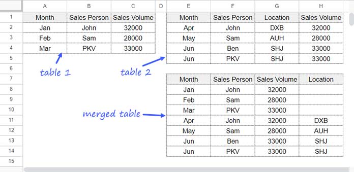
So, the number of columns is not the same. Also, the number of rows in the first table is 4, and the second table has 5 rows. How do we properly stack these tables vertically?

This type of merging is easier using HLOOKUP together with some other functions. Here are the step-by-step instructions.

Step 1: Merge Headers

To merge headers, you should first stack them horizontally and apply the UNIQUE function. Enter the following formula in cell E7:

=UNIQUE(HSTACK(A1:C1, E1:H1), TRUE)

The HSTACK function stacks the headers horizontally, and the UNIQUE function returns the distinct headers.

Step 2: Search Headers in Table #1 and Return Matching Rows

In cell E8, use this HLOOKUP formula:

=ArrayFormula(HLOOKUP(E7:H7, A1:C4, SEQUENCE(ROWS(A1:C4)-1, 1, 2), 0))

This follows the syntax HLOOKUP(search_key, range, index, [is_sorted]) where:

• search_key: E7:H7 (distinct headers)
• range: A1:C4 (table #1)
• index: SEQUENCE(ROWS(A1:C4)-1, 1, 2) (the row indices, dynamically generated)
• is_sorted: 0 (exact match)

We use ARRAYFORMULA because we have multiple search keys to look up.

Now, we need to merge the second table with the output of this HLOOKUP, which follows the same approach as above.

Step 3: Search Headers in Table #2 and Return Matching Rows

In cell E11, insert the following formula:

=ArrayFormula(HLOOKUP(E7:H7, E1:H5, SEQUENCE(ROWS(E1:H5)-1, 1, 2), 0))

It’s the same formula as in step 2, but with the table reference and row index changed.

Final Step: Combining Formulas

Combine the formulas into one to create a dynamic merge.

You can enter the following formula directly into cell E7. Before doing so, remove the step 1 – 3 formulas from the cells.

=ArrayFormula(LET(
   table_1, A1:C4, 
   table_2, E1:H5, 
   header, 
      UNIQUE(HSTACK(
         CHOOSEROWS(table_1, 1), 
         CHOOSEROWS(table_2, 1)
      ), TRUE), 
   IFNA(VSTACK(
      header, 
      HLOOKUP(header, table_1, SEQUENCE(ROWS(table_1)-1, 1, 2), 0), 
      HLOOKUP(header, table_2, SEQUENCE(ROWS(table_2)-1, 1, 2), 0)
   ))
))

In this formula, we use the LET function to name the tables and use those names in subsequent value expressions and formula expressions.

This approach ensures the merging is dynamic and handles tables with different numbers of columns and rows.

You just need to replace the table references A1:C4 and E1:H5 with the table references in your sheet. The formula handles the rest.

Merging Two Tables Using a Matching ID in Google Sheets

This is one of the most common types of merging.

Imagine you maintain separate tables for each month’s salaries of your employees. You might want to generate a report that shows their monthly salaries in one consolidated table.

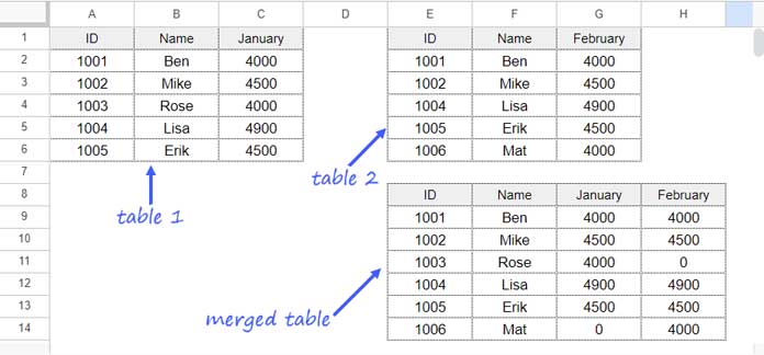
This involves merging two tables by stacking them horizontally. This method uses unique IDs (such as employee IDs) for merging.

Step 1: Merge Common Columns Including IDs

Based on our sample data, we aim to stack the salaries horizontally while matching the IDs. Aside from IDs, the common column in both tables is the name column.

To merge these columns from both tables, start by inserting the following formula into cell E9:

=UNIQUE(VSTACK(A2:B6, E2:F6))

The VSTACK function vertically stacks the IDs and Names from both tables, and the UNIQUE function returns distinct rows. This effectively merges the IDs and Names from both tables into one.

Step 2: Search Distinct IDs in Table #1 and Return Matching Columns

Insert the following VLOOKUP formula into cell G9 to retrieve the salaries from Table #1:

=ArrayFormula(IFNA(VLOOKUP(E9:E14, A1:C6, 3, 0), 0))

This follows the syntax VLOOKUP(search_key, range, index, [is_sorted]) where:

• search_key: E9:E14 (distinct IDs)
• range: A1:C6 (table #1)
• index: 3 (the column to return from table #1)
• is_sorted: 0 (exact match)

The IFNA function returns 0 if any ID doesn’t match in table #1.

Step 3: Search Distinct IDs in Table #2 and Return Matching Columns

Similar to step #2, use the following VLOOKUP formula in cell H9:

=ArrayFormula(IFNA(VLOOKUP(E9:E14, E1:G6, 3, 0), 0))

This method allows us to merge two tables by matching IDs in Google Sheets.

Resources

We have explored two methods to merge tables in Google Sheets. For advanced merging techniques, please refer to these guides:

• How to Left Join Two Tables in Google Sheets
• How to Right Join Two Tables in Google Sheets
• How to Inner Join Two Tables in Google Sheets
• How to Full Join Two Tables in Google Sheets
• Master Joins in Google Sheets (Left, Right, Inner, & Full) – Duplicate IDs Solved