In this detailed walkthrough, you’ll learn how to successfully perform a full join on two tables in Google Sheets.
A full join combines all records (rows) from both tables, regardless of whether they have matching values in a common field (column). It requires the presence of a unique identifier column in each table.
Matching records occupy the same row, while unmatched records from either table are included with missing values for corresponding fields in the other table.
Before proceeding, make sure:
- Both tables should have a unique identifier column. This column must contain distinct values for each record in the right table. This represents the most common scenario when joining two tables.
- The data types of the identifier columns in both tables are compatible. For example, both should be text, or both should be numbers.
Now, we’ll explore sample tables, expected results, the formula, and an explanation for performing a full join in Google Sheets.
Note: If you have duplicated IDs in both ID columns (left and right tables), please check out this guide: Conquer Duplicate IDs: Master Left, Right, Inner, & Full Joins in Google Sheets.
Full Join Two Tables: Sample Tables and Resulting Table
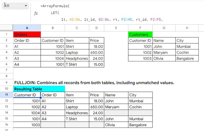
Orders (Left Table):
| Order ID | Customer ID | Item | Price |
| A1 | 1001 | Shirt | 18.00 |
| A2 | 1002 | Laptop | 650.00 |
| A3 | 1004 | Headphones | 24.00 |
| A4 | 1001 | T-Shirt | 15.00 |
Customers (Right Table):
| Customer ID | Name | City |
| 1001 | John | Mumbai |
| 1002 | Maryam | Cochin |
| 1003 | Olivia | Bangalore |
Expected Result of Full Join:
| Customer ID | Order ID | Item | Price | Name | City |
| 1001 | A1 | Shirt | 18.00 | John | Mumbai |
| 1002 | A2 | Laptop | 650.00 | Maryam | Cochin |
| 1004 | A3 | Headphones | 24.00 | – | – |
| 1001 | A4 | T-Shirt | 15.00 | John | Mumbai |
| 1003 | – | – | – | Olivia | Bangalore |
In this example, both tables share a common “Customer ID” column.
A full join combines all rows based on this shared identifier, including cases where some customers have no orders or some orders have no related customer information.
Array Formula for Full Joining Two Tables in Google Sheets
The following array formula performs a full join between two tables in Google Sheets. It assumes unique records in the right table.
Formula:
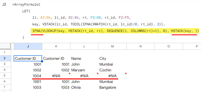
=ArrayFormula(
     LET(
          lt, A2:D6, lt_id, B2:B6, rt, F2:H5, rt_id, F2:F5,
          key, VSTACK(lt_id, TOCOL(IFNA(XMATCH(rt_id, lt_id)/0, rt_id), 3)),
          look_up, IFNA(VLOOKUP(key, HSTACK(rt_id, rt), SEQUENCE(1, COLUMNS(rt)+1), 0), HSTACK(key, )),
          IFNA(HSTACK(lt, look_up))
     )
)
Where:
A2:D6is the left table range, including the header row.B2:B6is the unique identifier column in the left table, including the field label.F2:H5is the right table range, including the header row.F2:F5is the unique identifier column in the right table, including the field label.
In the above formula, you need to replace IFNA(HSTACK(lt, look_up)) with CHOOSECOLS(IFNA(HSTACK(lt, look_up)), {5, 1, 3, 4, 7, 8}) to get a result similar to the resulting table above. This modification, specifically CHOOSECOLS, selects the required columns from the full join in the desired order.
Note: If any column in either of the two tables contains dates, you should format that column in the joined table as Format > Number > Date.
Check cell A11 of the fifth sheet in the provided sample sheet below for the full join array formula.
Formula Breakdown
To simplify the modification of the full join array formula, we’ve utilized the LET function.
The LET function assigns a name to a calculation result or a cell/range reference. This allows you to reuse those values within your formula without repeating the calculation or reference, improving both performance and readability.
Syntax of the LET Function:
LET(name1, value_expression1, [name2, …], [value_expression2, …], formula_expression)Assigned Range References
Here are the range references for the full Joining of two tables in Google Sheets:
lt(name1): Defines the data range of the left table (Orders), including the header row.A2:D6(value_expression1): Data range of the left table (Orders).
lt_id(name2): Defines the ID column of the left table (Orders), including the header row.B2:B6(value_expression2): ID column of the left table (Orders).
rt(name3): Defines the data range of the right table (Customers), including the header row.F2:H5(value_expression3): Data range of the right table (Customers).
rt_id(name4): Defines the ID column of the right table (Customers), including the header row.F2:F5(value_expression4): ID column of the right table (Customers).
Note: You only need to specify the above value_expressions 1 to 4 for your two tables. The full join array formula will take care of the rest.
Assigned Intermediate Calculation Results
VLOOKUP Keys: Search Keys for Full Join
key(name5): Defines the search keys for VLOOKUPVSTACK(lt_id, TOCOL(IFNA(XMATCH(rt_id, lt_id)/0, rt_id), 3))(value_expression5):
This “key” serves as a crucial element for performing a full join in Google Sheets. It vertically combines two components:
- All unique identifiers from the left table: This ensures all left table records are included in the join.
- Unique identifiers from the right table that are missing in the left table: This is achieved through a combination of XMATCH, error conversion, and IFNA.
- XMATCH locates and returns the index (position) of each right identifier within the left table. For unmatched values, it returns #N/A.
- Dividing the position by zero intentionally triggers matching IDs to return DIV/0! values.
- IFNA replaces #N/A values with the corresponding right identifiers.
- Finally, TOCOL converts this list of right-only identifiers into a single column.
By stacking (VSTACK) this “right-only” column with the left table identifiers, the “key” ensures all rows from both tables are included in the full join based on their unique ID presence.
VLOOKUP: The Soul of Full Joining Two Tables in Google Sheets
VLOOKUP is a crucial component of the full join between two tables in Google Sheets.
look_up(name6):IFNA(VLOOKUP(key, HSTACK(rt_id, rt), SEQUENCE(1, COLUMNS(rt)+1), 0), HSTACK(key, ))(value_expression6):
This part of the formula performs a lookup operation to retrieve data from the right table (rt) based on the key column created earlier. Let’s break it down step-by-step:
VLOOKUP(key, HSTACK(rt_id, rt), SEQUENCE(1, COLUMNS(rt)+1), 0)is the core lookup function.key: This is the column containing the combined unique identifiers from both tables (created by VSTACK earlier).HSTACK(rt_id, rt): This specifies the lookup range. This combines the right table identifier column (rt_id) with the right table (rt) horizontally.SEQUENCE(1, COLUMNS(rt)+1): Generates a range of numbers representing the column positions in the right table.0: This indicates an exact match is required for the lookup.
- IFNA:
- This function wraps the VLOOKUP to handle potential errors.
- If a match is found for a key in the right table, VLOOKUP returns the corresponding data from the lookup range (
HSTACK(rt_id, rt)). - If no match is found, VLOOKUP returns an array of #N/A errors, with the number of errors matching the size of the lookup range (number of columns).
- IFNA replaces any potential errors with a pattern derived from
HSTACK(key, ). This pattern replicates the key in the first cell and fills the remaining cells with NA values, matching the number of columns returned by VLOOKUP in the case of successful lookups.
Full Join Formula_Expression Part
This segment merges the data from the left table (lt) with the lookup result (look_up) and replaces #N/A (returned during stacking) with blanks.
IFNA(HSTACK(lt, look_up))Formula Breakdown:
HSTACK(lt, look_up): This part horizontally concatenates (stacks) the data from the left table (lt) with the lookup results (look_up) from the right table.IFNA(HSTACK(lt, look_up)): This wraps the preceding step with the IFNA function. This function replaces any potential errors encountered during the lookup with blank values.
Important Notes:
The lookup result includes all records from the right table. This ensures a full join, even for records with no matching information in the left table.
Wrapping this formula in CHOOSECOLS is necessary when the full join creates multiple unique identifier columns. This function allows you to select specific columns from the joined result, including just the key column you created.
E.g.: CHOOSECOLS(IFNA(HSTACK(lt, look_up)), {5, 1, 3, 4, 7, 8})


