Merging duplicate rows in Google Sheets can involve merging cell values, aggregating numbers, and concatenating text, dates, or timestamps.
Merging rows is the process of combining two or more rows of data that contain the same information. For example, two or more rows with the same first and last names, or the same product in more than one row.
In the case of combining two or more rows of data that contain the same product, you may need to add quantities or amounts to avoid losing data. We should consider all of this when coding formulas.
If you are looking for an array formula-based approach, without using any add-on, my following solution may be the best fit for you.
There is no built-in function or menu command to merge duplicate rows in Google Sheets in the way that we want.
To handle this, we will use three array formulas, each assigned to a specific task.
- The first array formula will remove duplicate rows (merging cells) in the data range in the specified columns.
- The second array formula will work as an alternative to the CONCATENATE function or JOIN function. It will join the removed rows’ values with the existing rows.
- The third array formula will conditionally sum columns. It will add the removed rows’ values to the existing rows.
Of course, you can merge cells (duplicates) using the UNIQUE function. What about aggregation and joining of values?
In fact, we can handle most of these tasks using the QUERY function itself. However, it falls short when it comes to joining or concatenating duplicates.
How to Merge Duplicate Rows in Google Sheets with an Example
In the following example, the source data for merging duplicate rows is in the cell range A2:E, and the results are in the cell range G2:K.
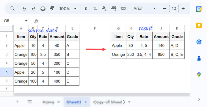
In merging the duplicate rows concept, first, we will remove duplicates in the Item column (A). This will give us unique fruit names (column G).
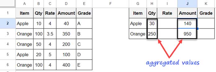
We will then sum the corresponding Qty in column (B) and the Amount in column (D) separately. The results are in columns H and J.
The Rate column (D) contains multiple rates for the same fruits. We will concatenate these rates for each fruit (column I). The Grade column (E) will be concatenated (joined) similarly. The results are in column K.
We will use three array formulas for each purpose, and repeat them, if necessary, for additional columns. This will allow anyone to adjust the ranges in the formula to customize the formula to their dataset.
Since the formulas are array formulas, we can use them with regular spreadsheet data, Google Form data in Sheets, as well as IMPORTRANGE data.
In this tutorial, you will get the array formulas for merging duplicate rows in Google Sheets. I will also explain how to use them.
Step 1: Unique to Merge Duplicate Cells
Syntax: UNIQUE(range, [by_column], [exactly_once])
In the above example of merging duplicate rows, the key column to merge is column A, which contains duplicate values (fruit names). Sometimes, you may have multiple columns that you want to merge. We will see that scenario later on.
We can use the UNIQUE function to unique the fruit names in column A. However, this is not enough. We should also include the FILTER function within the UNIQUE function. This is to filter out blank rows, because the UNIQUE function is infamous for returning a blank cell at the end.
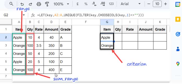
The following formula in cell G2 will unique the fruit names in column A and remove any blank cells:
=LET(key,A2:A,UNIQUE(FILTER(key,CHOOSECOLS(key,1)<>"")))When you use this formula, just replace A2:A with the corresponding column range.
Step 2: Aggregating Values while Retaining Removed Rows’ Values
Merging rows is more than just removing duplicate rows. We will remove the duplicate rows, but we will also keep the values in them with the retained row. If the values are text, date, time, or timestamp, we will combine them. But if the values are numbers, we may sum them or combine them, depending on our purpose.
How do we sum the values corresponding to the merged values in the first step?
We can use the SUMIF function for this. The syntax is SUMIF(range, criterion, [sum_range]).
In our sample data, the sum_range is B2:B, the range is A2:A and the criterion is the unique items in G2:G.
However, you don’t need to worry about the unique values (G2:G) in your formula. Just specify the range and sum_range, and the formula will take care of the rest.
H2 Formula:
=ARRAYFORMULA(LET(range,A2:A,sum_range,B2:B,SUMIF(TRANSPOSE(QUERY(TRANSPOSE(range),,9^9)),TRANSPOSE(QUERY(TRANSPOSE(UNIQUE(FILTER(range,CHOOSECOLS(range,1)<>""))),,9^9)),sum_range)))We can use the same resulting formula in cell J2 to sum the Amount column by replacing sum_range B2:B with D2:D.
=ARRAYFORMULA(LET(range,A2:A,sum_range,D2:D,SUMIF(TRANSPOSE(QUERY(TRANSPOSE(range),,9^9)),TRANSPOSE(QUERY(TRANSPOSE(UNIQUE(FILTER(range,CHOOSECOLS(range,1)<>""))),,9^9)),sum_range)))So, that is the second step of merging duplicate rows and concatenating values.
The above formula may seem complex but don’t worry about it. Just specify the ranges, and you’re good to go.
I have included some flexibility in the formula to adjust it automatically when you have multiple merge columns in Step 1 (G2 formula). We will see an example of this later on.
Step 3: Concatenating Values while Retaining Removed Rows’ Values
This is the third and final formula for merging duplicate rows and concatenating values.
In this step, we concatenate the Rates in the removed rows with the existing rates. This involves two columns: the column used to identify the unique rows in step 1, and the rate column.
Here is the I2 formula:
=LET(merge,A2:A,combine,C2:C,MAP(TRANSPOSE(QUERY(TRANSPOSE(UNIQUE(FILTER(merge,CHOOSECOLS(merge,1)<>""))),,9^9)),LAMBDA(row,TEXTJOIN(", ",TRUE,FILTER(combine,TRANSPOSE(QUERY(TRANSPOSE(merge),,9^9))=row)))))To concatenate the Grade column, use the same formula but replace the range C2:C with E2:E.
K2 Formula:
=LET(merge,A2:A,combine,E2:E,MAP(TRANSPOSE(QUERY(TRANSPOSE(UNIQUE(FILTER(merge,CHOOSECOLS(merge,1)<>""))),,9^9)),LAMBDA(row,TEXTJOIN(", ",TRUE,FILTER(combine,TRANSPOSE(QUERY(TRANSPOSE(merge),,9^9))=row)))))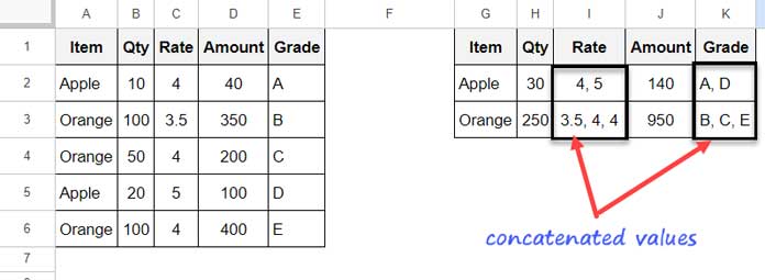
You have now the sets of 3 key formulas to merge duplicate rows in Google Sheets. Now let’s see a different dataset where we want to unique two columns.
Merging Duplicate Rows and Multiple Columns for Unique in Google Sheets
Here is the new sample data:
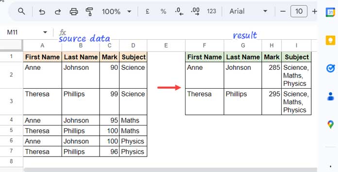
In this example, we want to merge the table based on the first and last names in columns A and B. The Mark should be aggregated and the Subject should be concatenated.
Here are the step-by-step instructions to merge duplicate first and last names and concatenate or aggregate corresponding columns:
- Scroll up and copy the formula under “Unique to Merge Duplicate Cells”. Replace the range A2:A with A2:B. Insert that formula in cell F2.
- Similarly, copy the first formula under “Aggregating Values while Retaining Removed Rows’ Values”. Replace A2:A with A2:B and B2:B with C2:C.
- Then, copy the first formula under “Concatenating Values while Retaining Removed Rows’ Values”. Replace A2:A with A2:B and C2:C with D2:D.
That’s it! You can use the above three formulas to merge duplicate rows in Google Sheets.


I’m trying to create a “Master List” of data between multiple sheets, but also need to merge duplicate rows and concatenate values. What is the best way to achieve “Point 1.1”?
For Reference, my data is currently listed on 8 separate sheets, columns A-S.
I want to group the duplicate information, that will be listed in column D-E, and concatenate the text values of column B.
Any advice is greatly appreciated.
Hi, JGibson,
If possible create a two-three tab example Sheet with mockup data. Also, wish to see the result that you are expecting.
Thank you very much Prashanth, you are awesome!