In this tutorial, I will guide you through the process of merging and unmerging cells in Google Sheets while also preserving values.
I understand that this is a straightforward task, with the exception of preserving values, and many of you may already be familiar with it. I’ve previously covered this as part of another Google Sheets formula tip.
To make this tutorial more engaging, I’ve included some formula tips to help you retain all the values within the merged area, which you might otherwise lose.
Introduction to Merging Cells in Google Sheets
I don’t recommend working with spreadsheets containing many merged cells. They can significantly hinder the data manipulation capabilities of Google Sheets or the spreadsheet program you are using.
In the case of Google Sheets, there are several functions that may not work well with datasets that include vertically or horizontally merged cells. Functions like DGET, SORT, QUERY, SUMIF, and FILTER are examples of this.
Additionally, menu commands such as ‘Sort,’ ‘Filter,’ and ‘Randomize Range’ within the ‘DATA’ menu may not work or may produce incorrect results.
Let me provide an example.
I have four names in column B and their corresponding sales quantities in column C.
When I attempted to sum the sales of “Brendan,” I used the following SUMIF formula:
=SUMIF(B3:B12, E3, C3:C12)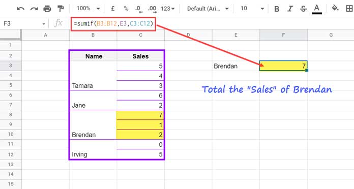
However, it returned 7 instead of 10. The discrepancy arises from the fact that the SUMIF criteria in cell E3 found a match in cell B8. Cells B9 and B10 do not contain the name “Brendan.” These cells are part of the merged range B8:B10, and as a result, their corresponding values weren’t included in the sum.
You can address these issues by virtually filling merged cells in formulas, but that’s a separate topic. In this tutorial, we will focus on how to merge and unmerge cells in Google Sheets.
Merging Cells in Google Sheets: Exploring Different Merge Types
To merge cells in Google Sheets, please follow the steps below:
- Select the cells you want to merge.
- Then, go to the ‘Format’ menu, and under ‘Merge cells,’ select one of the available merge options:
- Vertically: Choose this option when you have cells selected in a column.
- Horizontally: Select this option when you have cells selected in a row.
- Merge all: Use this option when you have cells selected in multiple rows and columns.
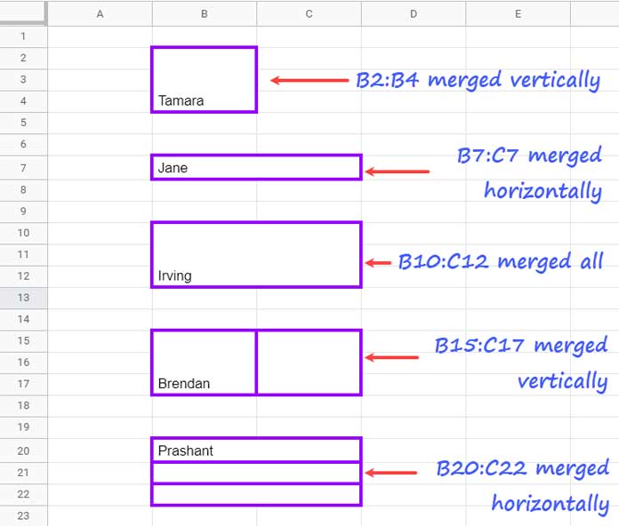
It’s important to note that in the case of ‘Merge all,’ where you have cells selected in multiple rows and columns, you can also choose either vertical or horizontal merging. This means there are a total of five merge types available.
Explaining Five Merge Types
Please refer to the screenshot below for a visual illustration.
In addition to the aforementioned Format menu commands, you can use shortcuts as well as a toolbar icon to merge cells in Google Sheets.
Keyboard Shortcuts (Windows):
- Alt + O + M + V: Merge Vertically
- Alt + O + M + H: Merge Horizontally
- Alt + O + M + A: Merge All
On Mac, you should replace ‘Alt’ with ‘Ctrl + Option.’
The toolbar icon is located just next to the ‘Borders’ icon, which may be initially faded out. To use this toolbar icon, first select more than one cell.
Merging Cells in Google Sheets: Preserving All Values
Below, you can learn how to merge cells Vertically, Horizontally, and with Merge All in Google Sheets while also preserving values.
Assume you have multiple values in the selected cells. When you merge cells in Google Sheets, it will only preserve the top-leftmost value. Google Sheets will alert you about this limitation.
This rule applies to all five of the aforementioned merge types.
What is the solution to this issue?
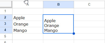
To preserve values, you can use formulas. For example, if you have values in cells A2:A3 and want to merge them into a single cell, use a formula in another similarly sized merged range, like cells B2:B3.
Insert the following TEXTJOIN formula in cell B2:
=TEXTJOIN(CHAR(10), TRUE, A2:A4)Right-click on cell B2 to open the shortcut menu and click ‘Copy.’ Then, open the shortcut menu again and select ‘Paste Special’ > ‘Values only.’
Delete the values in cells A2:A4. You can follow this method for all five merge types to preserve values.
Below are the formulas to preserve all the values in the selected cells when you merge cells in Google Sheets using any of the five methods mentioned above.
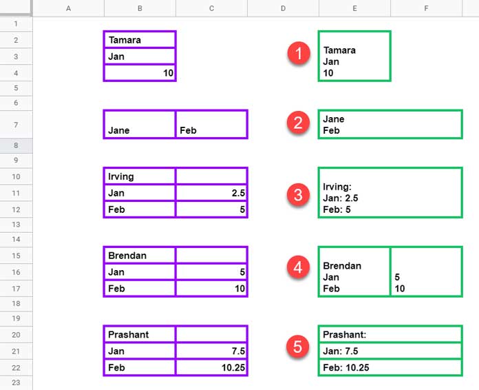
1. Merging in a Single Column
The range to merge is B2:B4.
In cell E2, enter the following TEXTJOIN formula. The delimiter in this formula is a new line character expressed by CHAR(10).
=TEXTJOIN(CHAR(10), TRUE, B2:B4)Select E2:E4, then go to ‘Format’ > ‘Merge cells’ > ‘Merge vertically.’
2. Merging in a Single Row
The range to merge is B7:C7.
In cell E7, enter the following formula, following the logic explained earlier:
=TEXTJOIN(CHAR(10), TRUE, B7:C7)Select E7:F7, then go to ‘Format’ > ‘Merge cells’ > ‘Merge horizontally.’
3-5. Merging Multiple Rows and Columns in the Merge Range
3. Merge All:
The range to merge is B10:C12.
In cell E10, enter the following formula, which utilizes the functions ArrayFormula and TEXTJOIN.
ArrayFormula is used due to the presence of the ampersand:
=ArrayFormula(TEXTJOIN(CHAR(10), TRUE, B10:B12 & ": " & C10:C12))Select E10:F12, then go to ‘Format’ > ‘Merge cells’ > ‘Merge all.
4. Vertically:
The range is B15:C17.
In cell E15, enter the nested TEXTJOIN formula below, which also utilizes the new line delimiter/string separator:
={TEXTJOIN(CHAR(10), TRUE, B15:B17), TEXTJOIN(CHAR(10), TRUE, C15:C17)}Select E15:F17, then go to ‘Format’ > ‘Merge cells’ > ‘Merge vertically.”
5. Horizontally:
The range is B20:C22.
In cell E20, enter the formula below:
=ArrayFormula(B20:B22&": "&C20:C22)Select E20:F22, then go to ‘Format’ > ‘Merge cells’ > ‘Merge horizontally.
Finally, select the range E2:F22. Right-click to open the shortcut menu, then choose ‘Copy.’ Right-click again, and this time, select ‘Paste Special’ and apply ‘Paste values.
After that, you can remove the values in B2:C22.
How to Unmerge Cells in Google Sheets
As I mentioned at the beginning of this Google Sheets tutorial, I don’t prefer spreadsheets with merged cells. If I receive a sheet with merged cells, I usually unmerge them promptly.
I find it more comfortable to work with sheets that don’t have this type of formatting.
So, how do you unmerge cells in Google Sheets?
Select the merged cells and go to ‘Format’ > ‘Merge cells’ > ‘Unmerge.’ You can also use the corresponding toolbar icon.
In the example above (screenshot #4), you can select E2:E4 and unmerge them as described.
But what if you need to unmerge multiple sets of merged cells in Google Sheets?
It’s a bit trickier. You should select multiple merged cells as follows:
- Click on the merged cell in the top row, as shown in the example (E2).
- Press and hold the Shift key.
- Click the merged cell in the last row, as shown in the example (E23).
Then go to ‘Format’ > ‘Merge cells’ > ‘Unmerge.’
Resources:


Hi Prashanth,
The use case that led me to your article, which is missing from it, is the scenario where you want to UNMERGE cells while preserving the value within and duplicating it across all the cells that are now unmerged.
Do you have any insights on that?
Hi Jerome,
You can search for the keyword “filling merged cells” within this post to find the linked tutorial.
Any way to merge/unmerge cells formulaically?
Hi, Helman,
I think there is no such option available in Sheets.